Czech record-level mortality data by vaccination status (part 3) - sars2.net

Links to other parts: czech.html, czech2.html, czech4.html.

Contents

People who were indicated to have a chronic illness

Uncle John Returns posted the tables below on Twitter and wrote: "Turns out that those Czechs who received a dose of Moderna in 2021 were twice as likely to have a pre-existing chronic condition as those who had Pfizer with AZ higher still. [...] The source is a ministry of health file which 
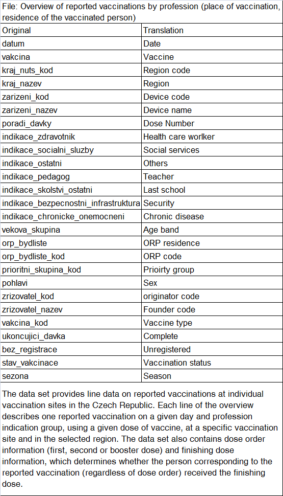
has 1 row per dose (so 3.68 GB) with other data such as the age band, sex and place of residence. Available on the vaccinations tab here https://onemocneni-aktualne.mzcr.cz/api/v2/covid-19." [https://x.com/UncleJo46902375/status/1814375808062112215]

The value of the indikace_chronicke_onemocneni column (indication chronic illness) is always either 1 or empty. I thought that the percentage of people where the value of the "indication chronic illness" column was 1 was surprisingly low, because there's only one age group where the column is true for over 10% of people with a first dose, and the percentage seemed to be fairly high in young age groups relative to old age groups (and for some reason it's about 10 times higher in ages 65-69 than ages 80+):

> download.file("https://onemocneni-aktualne.mzcr.cz/api/v2/covid-19/ockovani-profese.csv","ockovani-profese.csv") # about 4 GiB
> pro=fread("ockovani-profese.csv")
> d=pro[poradi_davky==1&vekova_skupina!="nezařazeno",.(.N,chronic=sum(indikace_chronicke_onemocneni,na.rm=T)),.(type=vakcina,age=as.numeric(sub("[+-].*","",vekova_skupina)))]
> d[,.(chronicpct=round(sum(chronic)/sum(N)*100,1)),age][order(age)]|>print(r=F)
 age chronicpct
   0        1.5
   5        0.0
  12        0.1
  16        0.6
  18        1.3
  25        1.7
  30        1.9
  35        2.4
  40        3.0
  45        3.9
  50        5.1
  55        6.6
  60        8.6
  65       11.1
  70        5.3
  75        2.1
  80        1.1

Clare Craig said that the column didn't mean if the person had a chronic illness or not but that it referred to "individuals preferentially vaccinated due to chronic disease", even though she didn't cite any source for why that would be the case. [https://drclarecraig.substack.com/p/double-checking-the-claims-about] That might explain why the total percentage of people who have the indication of a chronic illness is so low.

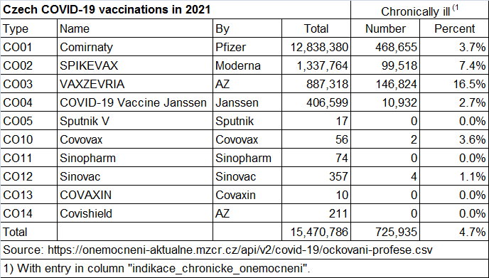
On this page for Czech vaccination statistics, there's 285,232 vaccinated people who have the "indication" of chronic illness (which is identical to the number of rows in the ockovani-profese.csv file where the indikace_chronicke_onemocneni column is true and the dose number is 1): https://ockovani.opendatalab.cz/statistiky_ockovani#ockovani-indikace. But there are also 273,374 vaccinated people who are in the "priority group" for a chronic illness. I don't know how the priority group is different from the indication group. A tooltip for the indication of chronic illness included the following text in Czech: "Chronically ill (hemato-oncological disease, oncological disease (solid tumors), serious acute or long-term heart disease, serious long-term lung disease, diabetes mellitus, obesity, serious long-term kidney disease, serious long-term liver disease, status after transplantation or on the waiting list, hypertension, seriousltip neurological or neuromuscular disease, congenital or acquired cognitive deficit, rare genetic disease, severe weakening of the immune system, other serious diseases)." But the tooltip for the priority group of chronic illness simply said "A person with a chronic illness".

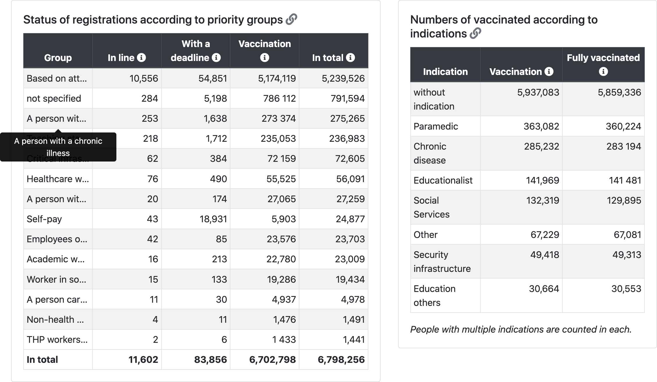
One explanation for why there's so few people who have the indication of chronic illness might be if they only include serious chronic illnesses. But it wouldn't explain why the percentage of people with an indication for chronic illness is much lower in ages 80+ than in ages 65-69. And the list of chronic illnesses in the tooltip also included hypertension, which alone should have a prevalence of more than the total percentage of people with the "indication" of chronic illness.

I found this PDF file which describes the "infectious disease information system" that is used in the Czech Republic ("Informační systém infekční nemoci", ISIN): https://vladci.cz/archive/covid/106/UZIS_2022-02_Struktura_NZIS_106.pdf. The PDF includes a list of fields which are contained in a database for COVID-19 cases, which also includes a module for COVID vaccinations. Here's a translation of the complete list of the so-called indications that were included in the vaccination module:

Indications (may change with regard to indications in the Central Reservation System - CRS):

In the file ockovani-registrace.csv which contains one row for each vaccinated person, there's a column called povolani (profession) which has the following values:

Count Translation Czech
6037598 Based on age Na základě dosaženého věku
912596 not specified neuvedeno
305888 A person with a chronic illness Osoba s chronickým onemocněním
275259 Teaching staff/non-teaching staff Pedagogický pracovník/nepedagogický zaměstnanec
79837 Critical infrastructure Kritická infrastruktura
70863 Healthcare worker according to §76 and §77 of Act 372/2011 Coll. Zdravotnický pracovník dle §76 a §77 zákona 372/2011 Sb.
39777 Self-paying Samoplátce
30231 A person with a chronic disease - in the care of a specialized center Osoba s chronickým onemocněním - v péči specializovaného centra
26026 Employees of the Ministry of Defense Zaměstnanci Ministerstva obrany
25530 University academic worker Akademický pracovník VŠ
21521 Worker in social services Pracovník v sociálních službách
5486 A person caring for a person in 3rd or 4th degree of dependence Osoba pečující o osobu v III. nebo IV. stupni závislosti
1813 Non-health care workers involved in the provision of health care and care
for COVID-19 positive persons
Nezdravotničtí pracovníci podílející se na poskytování zdravotní péče
a péče o covid-19 pozitivní osoby
1602 THP workers in hospitals THP pracovníci v nemocnicích

The values of the column might indicate the criteria based on which a person qualified to be vaccinated. By far the most common value of the column was by age. So if for example a person who was chronically ill qualified to be vaccinated because of their age, maybe only the qualification for age but not chronic illness was listed in the column, since each person has only one value listed in the column. So if a similar system was used in the ockoni-profese.csv file, it might explain why there's such a low percentage of people who are indicated to have a chronic illness in the oldest age groups.

In the table above the number of people with a chronic illness is 305,888 along with 30,231 people with a chronic illness who were in the care of a specialized center, so it's a bit higher than the file ockoni-profese.csv where there's rows for 285,232 first doses where the indikace_chronicke_onemocneni column is true (even though maybe there would be more unique people where the column would be true for at least one dose, but it's not possible to tell because the file doesn't have a way to identify which doses belong to the same person).

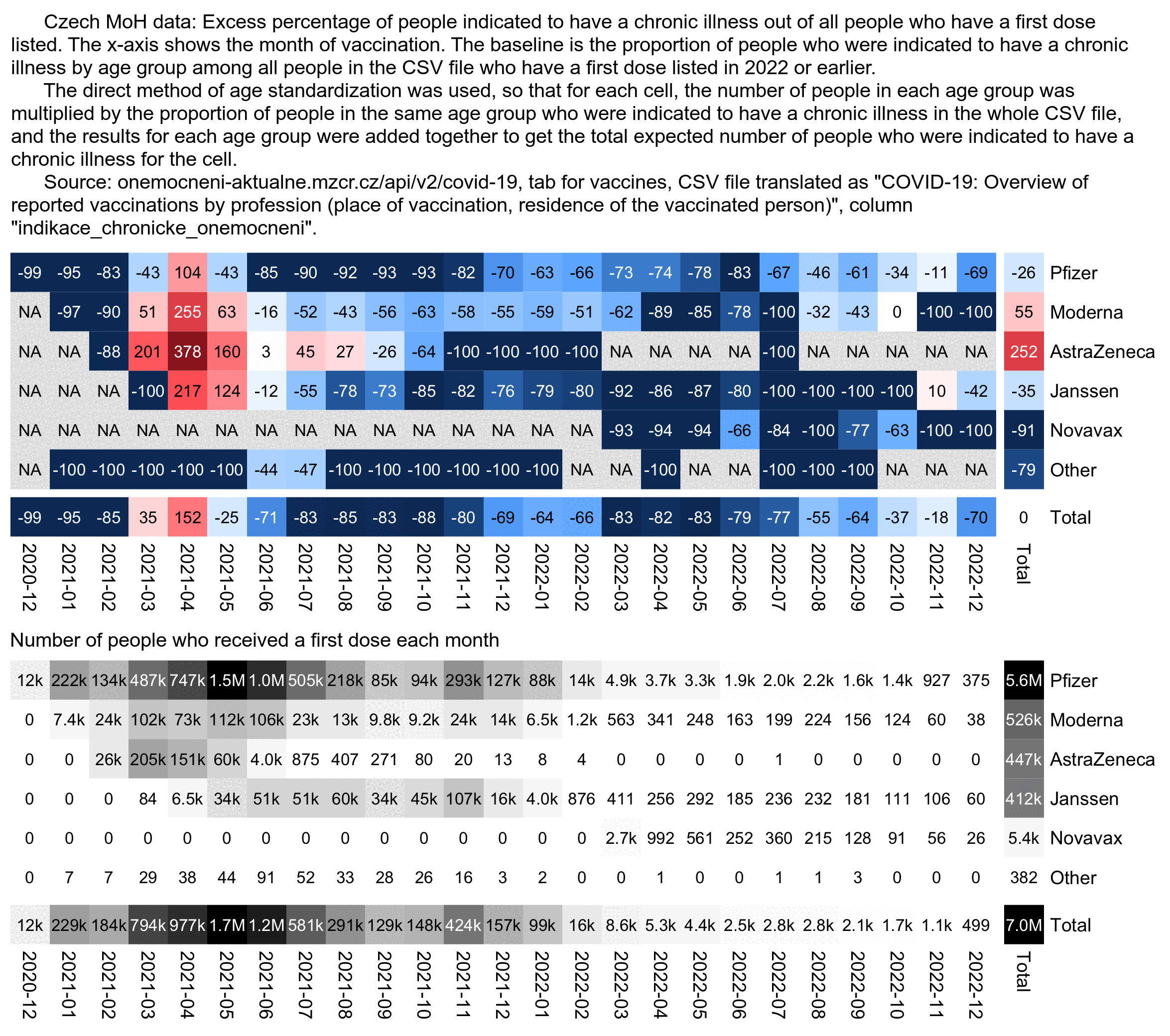
But anyway, in the following code I calculated an age-normalized proportion of people whose "indication chronic illness" column was true, so that my baseline was the proportion of the column by age group among all people who are included in the CSV file. The excess proportion of the column was about -26% for the first dose type Comirnaty but about 55% for SPIKEVAX:

> a=d[,.(N=sum(N),chronic=sum(chronic)),.(age,type)]
> a=merge(a,d[,.(base=sum(chronic)/sum(N)),age])[,base:=base*N]
> a[,.(pct=round((sum(chronic)/sum(base)-1)*100),N=sum(N)),type][order(-N)]|>print(r=F)
                                      type  pct       N
                                 Comirnaty  -26 5527776 # Pfizer
                                  SPIKEVAX   55  526448 # Moderna
                                 VAXZEVRIA  252  447428 # AstraZeneca
                  COVID-19 Vaccine Janssen  -35  412320
                            Comirnaty 5-11   31   59001
                                 Nuvaxovid  -91    5424 # Novavax
                Comirnaty Omicron XBB.1.5.    6    1988
      Comirnaty Original/Omicron BA.4/BA.5  -33     669
           Comirnaty Original/Omicron BA.1   77     294
                                   Sinovac  -72     181
                                Covishield -100     117
                            Comirnaty 6m-4 -100     111
           Comirnaty Omicron XBB.1.5. 5-11  -31     102
                                 Sinopharm -100      38
            COMIRNATY OMICRON XBB.1.5 6m-4  150      29
                                   Covovax  -33      29
   Spikevax bivalent Original/Omicron BA.1 -100      15
                                 Sputnik V -100      10
                         Nuvaxovid XBB 1.5 -100       8
                                   COVAXIN -100       5
 SPIKEVAX BIVALENT ORIGINAL/OMICRON BA.4-5  310       5
                                   Valneva -100       2
                                      type  pct       N

The next plot shows the age-normalized proportion of the column by vaccine type and month of vaccination. I was expecting the late vaccinees who got the first dose in late 2021 to have a higher age-normalized proportion of the "indication chronic illness" column than people who got vaccinated during the rollout peak, but actually I got the opposite result. However it might be if the indication for a chronic illness was generally not entered for people who qualified to be vaccinated based on other criteria such as age.

# download.file("https://onemocneni-aktualne.mzcr.cz/api/v2/covid-19/ockovani-profese.csv","ockovani-profese.csv")

library(data.table)

t=fread("ockovani-profese.csv")

yemo=\(x){u=unique(x);format(u,"%Y-%m")[match(x,u)]}

name1=unique(t$vakcina);name2=rep("Other",length(name1))
name2[name1==""]=""
name2[grep("comirnaty",ignore.case=T,name1)]="Pfizer"
name2[grep("spikevax",ignore.case=T,name1)]="Moderna"
name2[grep("nuvaxovid",ignore.case=T,name1)]="Novavax"
name2[name1=="COVID-19 Vaccine Janssen"]="Janssen"
name2[name1=="VAXZEVRIA"]="AstraZeneca"
t$type=name2[match(t$vakcina,name1)]

d=t[year(datum)<=2022&poradi_davky==1,.(.N,chronic=sum(indikace_chronicke_onemocneni,na.rm=T)),.(
  month=yemo(datum),type,age=vekova_skupina)][age!="nezařazeno"]

a=d[,.(N=sum(N),chronic=sum(chronic)),.(age,type,month)]
a=merge(a,d[,.(base=sum(chronic)/sum(N)),age])[,base:=base*N]
a=a[,.(chronic=sum(chronic),N=sum(N),base=sum(base)),.(type,month)]

a[,type:=factor(type,names(sort(a[,tapply(N,type,sum)],T)))]
a=rbind(a,a[,.(chronic=sum(chronic),N=sum(N),base=sum(base),month="Total"),type])
a=rbind(a,a[,.(chronic=sum(chronic),N=sum(N),base=sum(base),type="Total"),month])

m1=a[,tapply(chronic,.(type,month),c)]
m2=a[,tapply(base,.(type,month),c)]
pop=a[,xtabs(N~type+month)]

m=(m1-m2)/ifelse(m1>m2,m2,m1)*100
disp=round((m1/m2-1)*100)
exp=.82;maxcolor=500
m[m==-Inf]=-maxcolor

pheatmap::pheatmap(abs(m)^exp*sign(m),filename="i1.png",display_numbers=disp,
  gaps_row=nrow(m)-1,gaps_col=ncol(m)-1,
  cluster_rows=F,cluster_cols=F,legend=F,cellwidth=19,cellheight=19,fontsize=9,fontsize_number=8,
  border_color=NA,na_col="gray90",
  number_color=ifelse((abs(m)^exp>.55*maxcolor^exp)&!is.na(m),"white","black"),
  breaks=seq(-maxcolor^exp,maxcolor^exp,,256),
  colorRampPalette(hsv(rep(c(7/12,0),5:4),c(.9,.75,.6,.3,0,.3,.6,.75,.9),c(.4,.65,1,1,1,1,1,.65,.4)))(256))

kimi=\(x){e=floor(log10(ifelse(x==0,1,abs(x))));e2=pmax(e,0)%/%3+1;p=!is.na(x)
  x[p]=paste0(sprintf(paste0("%.",ifelse(e[p]%%3==0,1,0),"f"),x[p]/1e3^(e2[p]-1)),c("","k","M","B","T")[e2[p]]);x}

exp2=.6;maxcolor2=max(pop[-nrow(pop),-ncol(pop)])

pheatmap::pheatmap(pop^exp2,filename="i2.png",display_numbers=ifelse(pop<=10,round(pop),kimi(pop)),
  gaps_row=nrow(m)-1,gaps_col=ncol(m)-1,
  cluster_rows=F,cluster_cols=F,legend=F,cellwidth=19,cellheight=19,fontsize=9,fontsize_number=8,
  border_color=NA,na_col="white",
  number_color=ifelse(pop^exp2>maxcolor2^exp2*.45,"white","black"),
  breaks=seq(0,maxcolor2^exp2,,256),
  sapply(seq(1,0,,256),\(i)rgb(i,i,i)))

cap="\u00a0     Czech MoH data: Excess percentage of people indicated to have a chronic illness out of all people who have a first dose listed. The x-axis shows the month of vaccination. The baseline is the proportion of people who were indicated to have a chronic illness by age group among all people in the CSV file who have a first dose listed in 2022 or earlier.
      The direct method of age standardization was used, so that for each cell, the number of people in each age group was multiplied by the proportion of people in the same age group who were indicated to have a chronic illness in the whole CSV file, and the results for each age group were added together to get the total expected number of people who were indicated to have a chronic illness for the cell.
      Source: onemocneni-aktualne.mzcr.cz/api/v2/covid-19, tab for vaccines, CSV file translated as \"COVID-19: Overview of reported vaccinations by profession (place of vaccination, residence of the vaccinated person)\", column \"indikace_chronicke_onemocneni\"."
system(paste0("w=`identify -format %w i1.png`;pad=20;magick -pointsize 40 -font Arial \\( -size $[w-pad*3]x caption:'",cap,"' -splice $[pad]x20 \\) \\( i1.png -crop -0+8 \\) \\( -size $[w-pad*3]x caption:'Number of people who received a first dose each month' -splice $[pad]x0 \\) \\( i2.png -crop -0+8 \\) -append 1.png"))

system(paste0("w=`identify -format %w i1.png`;pad=20;magick -pointsize 40 -font Arial \\( -size $[w-pad*3]x caption:'",cap,"' -splice $[pad]x20 \\) \\( i1.png -crop -0+8 \\) \\( -size $[w-pad*3]x caption:'Number of people who received a first dose each month' -splice $[pad]x0 \\) \\( i2.png -crop -0+8 \\) -append 1.png"))

This shows the percentage of people by age group and vaccine type whose "indication chronic illness" column was true (where I again included only first doses):

> t=fread("ockovani-profese.csv")
> name1=unique(t$vakcina);name2=rep("Other",length(name1))
> name2[name1==""]=""
> name2[grep("comirnaty",ignore.case=T,name1)]="Pfizer"
> name2[grep("spikevax",ignore.case=T,name1)]="Moderna"
> name2[grep("nuvaxovid",ignore.case=T,name1)]="Novavax"
> name2[name1=="COVID-19 Vaccine Janssen"]="Janssen"
> name2[name1=="VAXZEVRIA"]="AstraZeneca"
> t$type=name2[match(t$vakcina,name1)]
> a=t[poradi_davky==1&vekova_skupina!="nezařazeno",.(.N,chronic=sum(indikace_chronicke_onemocneni,na.rm=T)),.(type,age=as.integer(sub("[-+].*","",vekova_skupina)))]
> a[,age:=factor(age,unique(age)[order(as.numeric(sub("[-+].*","",unique(age))))])]
> a[,type:=factor(type,a[,sum(N),type][order(-V1)]$type)]
> a=rbind(a,a[,.(N=sum(N),chronic=sum(chronic),age="Total"),type])
> a=rbind(a,a[,.(N=sum(N),chronic=sum(chronic),type="Total"),age])
> a[,tapply(round(chronic/N*100),.(type,age),c)]
             0  5 12 16 18 25 30 35 40 45 50 55 60 65 70 75 80 Total
Pfizer       1  0  0  1  1  1  2  2  2  3  4  5  6  7  3  1  1     3
Moderna     NA NA  0  1  3  4  4  5  5  7  8 10 12 16  7  3  2     7
AstraZeneca NA NA NA 14 17 16 19 20 21 25 28 31 34 39 12  4  3    17
Janssen     NA NA  0  0  1  1  1  1  2  3  3  4  5  5  5  5  4     3
Novavax     NA NA  0  0  0  0  0  0  0  0  1  0  1  2  0  1  2     0
Other       NA  0 NA  0  0  0  0  0  0  3  0  8  0  4  0  0  0     1
Total        1  0  0  1  1  2  2  2  3  4  5  7  9 11  5  2  1     4

This shows third doses instead of first doses:

             0  5 12  16 18 25 30 35 40 45 50 55 60 65 70 75 80 Total
Pfizer       0  0  0   1  2  2  3  3  4  5  6  7  9 11  5  2  1     5
Moderna     NA NA  0   2  3  4  4  5  5  7  8 10 13 17  8  3  2     7
AstraZeneca NA NA NA  NA  0  0  0 12  9  9 16 33 28 30  3  6  5    12
Janssen     NA NA NA  NA  2  4  4  4  5  5  6  9  7  9  4  3  3     5
Novavax     NA NA  0 100  7  0  0  3  0  0  6  0  0  6  5  0 12     3
Other       NA NA NA  NA NA  0  0  0  0  0  0  0  0  0  0  0 NA     0
Total        0  0  0   1  2  3  3  3  4  5  6  8  9 12  6  2  1     5

In both of the tables above Novavax got a lower percentage than Pfizer, which might partially explain people with a Novavax vaccine have such low mortality.

When I looked at third doses instead of first doses and I aggregated Omicron and pediatric vaccine types together with the main vaccine type, my excess age-normalized proportion of the "indication chronic illness" column was about -6% for Pfizer but 38% for Moderna:

> a=t[,.(N=sum(N),chronic=sum(chronic)),.(age,type)]
> a=merge(a,d[,.(base=sum(chronic)/sum(N)),age])[,base:=base*N]
> a[,.(pct=round((sum(chronic)/sum(base)-1)*100),N=sum(N)),type][order(-N)]|>print(r=F)
        type  pct       N
      Pfizer   -6 3805345
     Moderna   38  569083
     Janssen   -5    2463
 AstraZeneca  134     433
     Novavax  -48     318
       Other -100      28

When I calculated a Moderna-Pfizer ratio for an age-normalized proportion of the chronic illness column grouped by the month of the first dose, the ratio remained at a fairly steady level of about 5 to 6 for people who were vaccinated in May to October 2021, but the ratio suddenly dropped to about 2.3 the next month and it remained around 1 to 1.5 for the next 4 months. So that might also partially explain why the Moderna-Pfizer mortality ratio dropped to around 1.0 in people who were vaccinated in the fourth quarter of 2021 (even though the drop in the mortality ratio was already in October and not November):

> a=d[,.(N=sum(N),chronic=sum(chronic)),.(age,type,month)]
> a=merge(a,d[,.(base=sum(chronic)/sum(N)),age])[,base:=base*N]
> a=a[,.(rat=sum(chronic)/sum(base)),.(type,month)]
> m=a[,tapply(rat,.(type,month),c)]
> round(m["Moderna",]/m["Pfizer",],2)
2020-12 2021-01 2021-02 2021-03 2021-04 2021-05 2021-06 2021-07 2021-08 2021-09
     NA    0.62    0.61    2.65    1.74    2.87    5.68    5.03    6.86    5.84
2021-10 2021-11 2021-12 2022-01 2022-02 2022-03 2022-04 2022-05 2022-06 2022-07
   5.44    2.32    1.51    1.12    1.45    1.40    0.43    0.67    1.35    0.00
2022-08 2022-09 2022-10 2022-11 2022-12 2023-01 2023-02 2023-03 2023-04 2023-05
   1.26    1.47    1.51    0.00    0.00    3.74    0.00    0.00    0.00     NaN
2023-06 2023-07 2023-08 2023-09 2023-10 2023-11 2023-12 2024-01 2024-02 2024-03
     NA      NA      NA    0.00    0.00    0.00    0.00    0.00      NA      NA
2024-04 2024-05 2024-06 2024-07
     NA      NA     NaN      NA

This shows the age-normalized chronic illness ratio compared to the age-normalized mortality ratio:

download.file("https://onemocneni-aktualne.mzcr.cz/api/v2/covid-19/ockovani-profese.csv","ockovani-profese.csv")
download.file("http://sars2.net/f/czbucketskeep.csv.gz","czbucketskeep.csv.gz")

library(data.table);library(ggplot2)

yemo=\(x){u=unique(x);format(u,"%Y-%m")[match(x,u)]}
kim=\(x)ifelse(x>=1e3,ifelse(x>=1e6,paste0(x/1e6,"M"),paste0(x/1e3,"k")),x)

t=fread("ockovani-profese.csv")

d=t[poradi_davky==1,.(.N,chronic=sum(indikace_chronicke_onemocneni,na.rm=T)),.(type=vakcina,age=vekova_skupina,month=yemo(datum))][age!="nezařazeno"]

name1=unique(d$type);name2=ifelse(name1=="","","Other")
name2[grep("comirnaty",ignore.case=T,name1)]="Pfizer"
name2[grep("spikevax",ignore.case=T,name1)]="Moderna"
name2[grep("nuvaxovid",ignore.case=T,name1)]="Novavax"
name2[name1=="COVID-19 Vaccine Janssen"]="Janssen"
name2[name1=="VAXZEVRIA"]="AstraZeneca"
d$type=name2[match(d$type,name1)]

a=d[,.(N=sum(N),chronic=sum(chronic)),.(age,type,month)]
a=merge(a,d[,.(base=sum(chronic)/sum(N)),age])[,base:=base*N]
a=a[,.(chronic=sum(chronic)/sum(base),N=sum(N)),.(type,month)]
p=dcast(a,month~type,value.var="chronic")[,.(month,chronic=Moderna/Pfizer)]
p=cbind(p,dcast(a,month~type,value.var="N")[,.(Pfizer,Moderna)])

b=fread("czbucketskeep.csv.gz")[,age:=pmax(pmin(95,age%/%5*5),15)]
me=merge(b[dose==1],b[dose<=1,.(base=sum(dead)/sum(alive)),age])[,base:=base*alive]
me=me[,.(rate=sum(dead)/sum(base)),.(month=vaxmonth,type)]
p=merge(p,dcast(me,month~type,value.var="rate")[,.(month,mort=Moderna/Pfizer)])

p1=data.frame(month=p$month,y=c(p$mort,p$chronic),type=rep(c("Mortality ratio","Chronic illness ratio"),each=nrow(p)))
p2=data.frame(month=p$month,y=c(p$Pfizer,p$Moderna),type=rep(c("Pfizer","Moderna"),each=nrow(p)))
p1$type=factor(p1$type,unique(p1$type))
p2$type=factor(p2$type,unique(p2$type))

cand=c(sapply(c(1,2,5),\(x)x*10^c(-10:10)))
ymax=max(p$chronic,p$mort,na.rm=T)
ystep=cand[which.min(abs(cand-ymax/6))]
yend=ystep*ceiling(ymax/ystep)
ymax2=max(p2$y,na.rm=T)
ystep2=cand[which.min(abs(cand-ymax2/6))]
yend2=ystep2*ceiling(ymax2/ystep2)
secmult=yend/yend2

pal1=c("black","gray60")
pal2=alpha(hsv(c(22,0)/36,1,.8),.5)

exp=.7;xstart=1-exp;xend=length(p$month)+exp

ggplot(p,aes(x=month))+
geom_vline(xintercept=c(xstart,xend),linewidth=.3,lineend="square")+
geom_hline(yintercept=1,linewidth=.3,linetype=2,lineend="square")+
geom_bar(data=p2,aes(y=y*secmult,fill=type),stat="identity",position="dodge",linewidth=.15)+
geom_line(data=na.omit(p1),aes(y=y,color=type,group=type),linewidth=.4)+
labs(title="Age-normalized Moderna-Pfizer ratio by month of vaccination",x=NULL,y="Moderna-Pfizer ratio")+
scale_x_discrete(expand=expansion(mult=0,add=exp))+
scale_y_continuous(limits=c(0,yend),breaks=seq(0,yend,ystep),expand=expansion(0),labels=\(x)ifelse(x>=1e3,paste0(x/1e3,"k"),x),sec.axis=sec_axis(trans=~./secmult,breaks=seq(0,yend2,ystep2),name="Monthly new doses",labels=kim))+
scale_color_manual(values=pal1)+
scale_fill_manual(values=pal2)+
coord_cartesian(clip="off")+
theme(axis.text=element_text(size=7,color="black"),
  axis.text.x=element_text(angle=90,vjust=.5,hjust=1,margin=margin(2.5)),
  axis.ticks=element_line(linewidth=.3),
  axis.ticks.length=unit(3,"pt"),
  axis.ticks.length.x=unit(0,"pt"),
  axis.title=element_text(size=7,color="black"),
  axis.title.y.left=element_text(margin=margin(,3,,1)),
  axis.title.y.right=element_text(margin=margin(,,,4)),
  legend.direction="horizontal",
  legend.background=element_rect(fill=alpha("white",0)),
  legend.box.spacing=unit(0,"pt"),
  legend.key.height=unit(4,"pt"),
  legend.key.width=unit(15,"pt"),
  legend.key=element_rect(fill=alpha("white",0)),
  legend.margin=margin(0,2,4,2),
  legend.position="top",
  legend.spacing.x=unit(2,"pt"),
  legend.text=element_text(size=7),
  legend.title=element_blank(),
  panel.grid.major=element_blank(),
  panel.background=element_rect(fill="white"),
  plot.margin=margin(4,4,4,4),
  plot.title=element_text(size=7.5,margin=margin(1,0,4.5,0),face=2))
ggsave("0.png",width=4,height=2.2,dpi=300*4)
system("magick 0.png -resize 25% 1.png")

This also shows the Moderna-Pfizer ratio for chronic illness by age group and month of vaccination:

Hospitalizations by vaccine type

The second file from the bottom under vaccinations here has data for hospitalizations by vaccine type and age group: https://onemocneni-aktualne.mzcr.cz/api/v2/covid-19.

The file has about 7 million rows with one row for each vaccinated person. It has these columns:

            kraj_bydliste_nazev name of region of resicence
              kraj_bydliste_kod code of region of residence
             orp_bydliste_nazev name of county of residence
               orp_bydliste_kod code of county of residence
               vekova_kategorie age category
           ockovaci_latka_nazev vaccine name
             ockovaci_latka_kod vaccine code
                    prvni_davka date of first dose
                    druha_davka date of second dose
             dokoncene_ockovani date when completed primary course
               posilujici_davka date of booster dose
        indikace_pred_ockovanim type of test before vaccination
        pozivita_pred_ockovanim positivity of test before vaccination
  pozivita_pred_ockovanim_datum date of positive test before vaccination
   hospitalizace_pred_ockovanim hospitalized before vaccination
             jip_pred_ockovanim ICU before vaccination
           indikace_po_ockovani type of test after vaccination
           pozivita_po_ockovani positivivity of test after vaccination
     pozivita_po_ockovani_datum date of positive test after vaccination
      hospitalizace_po_ockovani hospitalized after vaccination
                jip_po_ockovani ICU after vaccination

The types of test are diagnostic, preventative, epidemiological, or other (ostatní). Negative tests are not listed so the type of the test is only shown for positive tests. There's only up to one test before vaccination and one test after vaccination listed for each person, and similarly there's only up to one hospitalization before vaccination and one hospitalization after vaccination listed for each person.

I used the file to calculate an age-normalized hospitalization rate from the day of the first dose up to the present. I didn't account for aging of people over time, so I treated the age at vaccination as the age of each person. The file included data for hospitalizations up the the present month, so I used the date when I downloaded the file as the end of my observation period.

In order to calculate the expected number of deaths for each vaccine type, I multiplied the number of person-days the vaccine type had for each age group with the mortality rate of each age group among all people who had a first dose listed in the file.

My excess percentage of hospitalizations was about -6% for the first dose type "Comirnaty" and about -4% for the first dose type "SPIKEVAX", so there was not much difference, but AstraZeneca and particularly Janssen vaccines had a much higher excess hospitalization rate:

> download.file("https://onemocneni-aktualne.mzcr.cz/api/v2/covid-19/ockovani-pozitivni-hospitalizovani.csv","ockovani-pozitivni-hospitalizovani.csv")
> h=fread("ockovani-pozitivni-hospitalizovani.csv")
> d=h[,.(age=vekova_kategorie,date=prvni_davka,type=ockovaci_latka_nazev,hosp=hospitalizace_po_ockovani)][age!="-"]
> maxdate=as.IDate("2024-7-20")
> a=d[,.(hosp=sum(hosp,na.rm=T),pop=sum(as.double(maxdate-date+1))),.(type,age)]
> a=merge(a,a[,.(base=sum(hosp)/sum(pop)),age])[,base:=base*pop]
> a[,.(excesspct=round((sum(hosp)/sum(base)-1)*100),hospitalizations=sum(hosp),pyears=round(sum(pop/365))),type][order(-pyears)]|>print(r=F)
                                      type excesspct hospitalizations   pyears
                                 Comirnaty        -6            43053 17432607 # Pfizer
                                  SPIKEVAX        -4             6234  1657122 # Moderna
                                 VAXZEVRIA        19            11921  1478098 # AstraZeneca
                  COVID-19 Vaccine Janssen        57             3576  1185707
                                 Nuvaxovid       -50                7    12140 # Novavax
                Comirnaty Omicron XBB.1.5.       -10                7     1349
      Comirnaty Original/Omicron BA.4/BA.5      -100                0     1015
                                   Sinovac      -100                0      543
           Comirnaty Original/Omicron BA.1      -100                0      454
                                Covishield      -100                0      372
                            Comirnaty 6m-4      -100                0      143
                                 Sinopharm      -100                0      113
                                   Covovax      -100                0       87
           Comirnaty Omicron XBB.1.5. 5-11      -100                0       62
                                 Sputnik V      -100                0       30
   Spikevax bivalent Original/Omicron BA.1      -100                0       22
                                   COVAXIN      -100                0       16
            COMIRNATY OMICRON XBB.1.5 6m-4      -100                0       15
 SPIKEVAX BIVALENT ORIGINAL/OMICRON BA.4-5      -100                0        4
                                   Valneva      -100                0        4
                         Nuvaxovid XBB 1.5      -100                0        2
                                      type excesspct hospitalizations   pyears

In the code below I additionally normalized the hospitalization rate for the month of vaccination. I now only included first doses given in 2021, because otherwise I would've been more likely to get anomalously high baseline mortality rates for combinations of vaccination month and age group that had a low number of person-days. However now Moderna got a slightly lower excess hospitalization percent than Pfizer which was the opposite of my previous calculation. And now the excess hospitalization percent of Janssen vaccines approximately halved from 57% to 28%, because late vaccinees had a higher hospitalization rate than early vaccinees and late vaccinees were overrepresented for Janssen vaccines:

> yemo=\(x){u=unique(x);format(u,"%Y-%m")[match(x,u)]}
> d2=d[date<="2021-12-31"][,month:=yemo(date)]
> a=d2[,.(hosp=sum(hosp,na.rm=T),pop=sum(as.double(maxdate-date+1))),.(type,age,month)]
> a=merge(a,a[,.(base=sum(hosp)/sum(pop)),.(month,age)])[,base:=base*pop]
> a=a[,.(excesspct=round((sum(hosp)/sum(base)-1)*100),hospitalizations=sum(hosp),pyears=round(sum(pop/365))),type]
> a[order(-pyears)]|>print(r=F)
                     type excesspct hospitalizations   pyears
                Comirnaty        -5            42775 17127673
                 SPIKEVAX        -6             6210  1633228
                VAXZEVRIA        21            11921  1478067
 COVID-19 Vaccine Janssen        28             3562  1168387
                  Sinovac      -100                0      539
               Covishield      -100                0      372
                Sinopharm      -100                0      109
                  Covovax      -100                0       85
                Sputnik V      -100                0       28
                  COVAXIN      -100                0       16

The next plot shows the excess hospitalization percent by age and the month of the first dose. There's a diagonal pattern across different age groups where there's a low excess hospitalization percent during the same month when the number of first doses peaked in the age group:

The next plot shows the excess hospitalization rate by vaccine type instead of age group. Janssen and AstraZeneca got a much higher total hospitalization rate than Pfizer and Moderna. I didn't normalize the total excess mortality by the month of vaccination so Janssen again got a very high total percentage of excess hospitalizations (because the late vaccinees who had a high hospitalization rate were overrepresented for Janssen vaccines):

Here's code for making the heatmaps:

library(data.table)

h=fread("ockovani-pozitivni-hospitalizovani.csv")

d=h[,.(age=vekova_kategorie,date=prvni_davka,type=ockovaci_latka_nazev,hosp=hospitalizace_po_ockovani)]
d=d[age!="-"&date<"2022-01-01"]
u=unique(d$date);d$month=format(u,"%Y-%m")[match(d$date,u)]

a=d[,.(.N,hosp=sum(hosp,na.rm=T),pop=sum(as.double(as.IDate("2024-7-20")-date+1))),.(month,age)]
a=merge(a,a[,.(base=sum(hosp)/sum(pop)),age])[,base:=base*pop]

p=a[,.(N=sum(N),hosp=sum(hosp),base=sum(base),pop=sum(pop)),.(month,age)]
p=rbind(p,p[,.(N=sum(N),hosp=sum(hosp),base=sum(base),pop=sum(pop),age="Total"),month])
p=rbind(p,p[,.(N=sum(N),hosp=sum(hosp),base=sum(base),pop=sum(pop),month="Total"),age])

m=p[,tapply((hosp-base)/ifelse(hosp>base,base,hosp)*100,.(age,month),c)]
disp=p[,tapply((hosp/base-1)*100,.(age,month),round)]
pop=p[,xtabs(N~age+month)]

exp=.7;maxcolor=300;m[m==-Inf]=-maxcolor

pheatmap::pheatmap(abs(m)^exp*sign(m),filename="i1.png",display_numbers=disp,
  gaps_row=nrow(m)-1,gaps_col=ncol(m)-1,
  cluster_rows=F,cluster_cols=F,legend=F,cellwidth=19,cellheight=19,fontsize=9,fontsize_number=8,
  border_color=NA,na_col="gray90",
  number_color=ifelse((abs(m)^exp>.55*maxcolor^exp)&!is.na(m),"white","black"),
  breaks=seq(-maxcolor^exp,maxcolor^exp,,256),
  colorRampPalette(hsv(rep(c(7/12,0),5:4),c(.9,.75,.6,.3,0,.3,.6,.75,.9),c(.4,.65,1,1,1,1,1,.65,.4)))(256))

kimi=\(x){e=floor(log10(ifelse(x==0,1,abs(x))));e2=pmax(e,0)%/%3+1;p=!is.na(x)
  x[p]=paste0(sprintf(paste0("%.",ifelse(e[p]%%3==0,1,0),"f"),x[p]/1e3^(e2[p]-1)),c("","k","M","B","T")[e2[p]]);x}

exp2=.6;maxcolor2=max(pop[-nrow(pop),-ncol(pop)])

pheatmap::pheatmap(pop^exp2,filename="i2.png",display_numbers=ifelse(pop<=10,round(pop),kimi(pop)),
  gaps_row=nrow(m)-1,gaps_col=ncol(m)-1,
  cluster_rows=F,cluster_cols=F,legend=F,cellwidth=19,cellheight=19,fontsize=9,fontsize_number=8,
  border_color=NA,na_col="white",
  number_color=ifelse(pop^exp2>maxcolor2^exp2*.45,"white","black"),
  breaks=seq(0,maxcolor2^exp2,,256),
  sapply(seq(1,0,,256),\(i)rgb(i,i,i)))

cap="\u00a0     Czech MoH data: Excess percentage for age-normalized hospitalization rate for people with a first dose listed in 2021. The x-axis shows the month of vaccination. The baseline is the hospitalization rate among people in the same age group in the CSV file who got a first dose in 2021. The hospitalization rate was calculated from the day of the first dose until July 20th 2024.
      Source: onemocneni-aktualne.mzcr.cz/api/v2/covid-19, tab for vaccinations, second file from bottom translated as \"COVID-19: Overview of persons with reported vaccinations with regard to SARS-CoV-2 infection\"."

system(paste0("pad=24;w=`identify -format %w i1.png`;magick -pointsize 40 -font Arial \\( -size $[w*2-pad*3] caption:'",cap,"' -splice $[pad]x20 \\) -font Arial-Bold \\( \\( \\( -size $[w-pad*3] caption:'Excess hospitalization percentage' -splice $[pad]x20 \\) i1.png -append \\) \\( \\( -size $[w-pad*2] caption:'Number of people who received a first dose each month' -splice $[pad]x20 \\) i2.png -append \\) +append \\) -append 1.png"))

Moderna-Pfizer ratio by weeks after vaccination

I have been telling Kirsch that if the reason why Moderna has higher ASMR than Pfizer would be because Moderna vaccines were killing a lot more people, you'd expect the Moderna-Pfizer ratio to be higher in the first days or weeks following vaccination and get closer to 1.0 over time, because deaths caused by vaccines would probably be much more common in the days or weeks following vaccination than more than a year after vaccination.

However this plot shows that the Moderna-Pfizer ratio remains at a consistent level of about 1.1 to 1.6 until it shoots up at the very end of the plot (when there's only a small number of people who got vaccinated early enough that they had not yet ran out of follow-up time):

In the black line the ratio was only normalized by age. In the gray line the ratio was additionally normalized by ongoing month, but it didn't change the results that much.

But anyway, you would at least think that there would be more vaccine deaths in weeks 0 to 29 after vaccination than in weeks 60 to 89. But because the Moderna-Pfizer ratio remains consistently elevated even more than a year after vaccination, it rather seems to be the product of some kind of confounding factors.

b=data.table::fread("http://sars2.net/f/czbucketskeep.csv.gz")
b[,age:=pmax(pmin(95,age%/%5*5),15)]

d=merge(b[dose==1],b[dose<=1,.(base2=sum(dead)/sum(alive)),.(month,age)])[,base2:=base2*alive]
d=merge(d,b[dose<=1,.(base1=sum(dead)/sum(alive)),age],by="age")[,base1:=base1*alive]
d=d[,.(rate1=sum(dead)/sum(base1),rate2=sum(dead)/sum(base2)),.(week,type)]

a1=d[,xtabs(rate1~week+type)];r1=a1[,"Moderna"]/a1[,"Pfizer"]
a2=d[,xtabs(rate2~week+type)];r2=a2[,"Moderna"]/a2[,"Pfizer"]
week=unique(d$week)

png("1.png",1300,800,res=198)
par(mar=c(2.3,2.3,2.1,.8),mgp=c(0,.6,0))
tit="Age-normalized Moderna-Pfizer ratio by weeks after first dose"
leg=c("Normalized by age only","Normalized by age and ongoing month")
col=c("black","gray60")
plot(week,r1,type="l",col=col[1],main=tit,xlab=NA,ylab=NA,lwd=1.5,cex.main=1.1)
abline(h=1,lty=2)
lines(week,r2,type="l",col=col[2],lwd=1.5)
legend("bottom",legend=leg,col=col,lty=1,lwd=1.5)
dev.off()

Efficacy against hospitalization relative to a baseline of unvaccinated people

The following code calculates an age-normalized excess hospitalization percentage relative to a baseline of unvaccinated people. The observation period starts in January 2021 and ends on July 20th 2024.

I combined two different CSV files published by the Czech Ministry of Health: https://onemocneni-aktualne.mzcr.cz/api/v2/covid-19.

I took hospitalizations by vaccine type from the same CSV file as earlier. It's missing the date of hospitalization but it only has a field which indicates if a person has been hospitalized after vaccination or not, so I had to calculate the hospitalization rate up to the present day and I wasn't able to choose which day my observation period ended.

I took hospitalizations in unvaccinated people from another CSV file published by the MoH. But I didn't find a good way to calculate the number of person-days for unvaccinated people up to the present day, so I took the number of person-days for unvaccinated people from one of my buckets files, so that I used the number of person-days in each age group in December 2022 as the subsequent population size up to July 2024 so that I adjusted the person-days for the length of each month.

system("wget onemocneni-aktualne.mzcr.cz/api/v2/covid-19/ockovani-{hospitalizace-tyden,pozitivni-hospitalizovani}.csv sars2.net/f/czbucketsdaily.csv.gz")

library(data.table)

yemo=\(x){u=unique(x);format(u,"%Y-%m")[match(x,u)]}

unvaxhosp=fread("ockovani-hospitalizace-tyden.csv")
unvax=unvaxhosp[,.(hosp=hospitalizovani_bez_ockovani),.(date=tyden_od+3,age=pmax(25,pmin(80,as.numeric(sub("[-+].*","",vekova_skupina)))))][,spline(date,hosp/7,xout=min(date):max(date)),age][,.(hosp=sum(y)),.(age,month=yemo(`class<-`(x,"Date")))]

maxdate=as.IDate("2024-7-20")

unvaxpop=fread("czbucketsdaily.csv.gz")[dose==0][,.(pop=sum(alive)),.(month=yemo(date),age=pmax(pmin(age,80),25)%/%5*5)]
unvaxpop=rbind(unvaxpop,unvaxpop[month=="2022-12",.(pop,month=seq(as.Date("2023-1-1"),as.Date("2024-7-1"),"month")),age][,pop:=pop/31*ifelse(month==as.Date("2024-7-1"),20,lubridate::days_in_month(month))][,month:=yemo(month)][])

vaxhosp=fread("ockovani-pozitivni-hospitalizovani.csv")
vax=vaxhosp[,.(age=vekova_kategorie,date=prvni_davka,type=ockovaci_latka_nazev,hosp=hospitalizace_po_ockovani)][age!="-"]

name1=unique(vax$type);name2=rep("Other",length(name1))
name2[name1==""]=""
name2[grep("comirnaty",ignore.case=T,name1)]="Pfizer"
name2[grep("spikevax",ignore.case=T,name1)]="Moderna"
name2[grep("nuvaxovid",ignore.case=T,name1)]="Novavax"
name2[name1=="COVID-19 Vaccine Janssen"]="Janssen"
name2[name1=="VAXZEVRIA"]="AstraZeneca"
vax$type=name2[match(vax$type,name1)]

a=vax[,.(hosp=sum(hosp,na.rm=T),pop=sum(as.double(as.IDate("2024-7-20")-date+1))),.(age=pmax(25,pmin(80,as.numeric(sub("[+-].*","",age)))),type)]

a=merge(a,merge(unvax,unvaxpop)[,.(hosp=sum(hosp),pop=sum(pop)),age][,.(base=hosp/pop,age)])[,base:=base*pop][]

a[,.(excess=(sum(hosp)/sum(base)-1)*100),type][order(-excess),excess:=round(excess)][]|>print(r=F)

I only considered first doses in the code above. The output shows that the excess hospitalization percent was about -79% for people whose first dose was Pfizer, -77% for Moderna, -71% for AstraZeneca, and -68% for Janssen:

        type excesspct
      Pfizer       -79
     Moderna       -77
     Novavax       -91
 AstraZeneca       -71
     Janssen       -68
       Other      -100

So in other words unvaccinated people had about 5 times higher age-normalized hospitalization rate than people who got a Pfizer vaccine for the first dose, or Pfizer vaccines had about 79% efficacy in preventing hospitalization relative to the baseline of unvaccinated people.

Novavax got an excess hospitalization percent of -91% above, but it's because people only started getting Novavax vaccines in March 2022 after which there weren't that many people hospitalized for COVID. The CSV file I used to get hospitalization data by vaccine type is missing the date of hospitalization, so I wasn't able to adjust my excess mortality percent for the ongoing month.

For the rare vaccine types that I aggregated under the label "Other", there were zero hospitalizations so the excess hospitalization percent was -100%.

But anyway, my results roughly seem to match the record-level data which shows that during the COVID wave in the last two months of 2021, the spike in all-cause ASMR was higher for Janssen and AstraZeneca vaccines but more flat for Moderna and Pfizer.

One limitation of my analysis is that a large part of the person-days of vaccinated people are during periods with low hospitalizations from mid-2022 up to July 2024 and in the third quarter of 2021. But unvaccinated people have a lot of person-days in the first quarter of 2021 when there was a high number of hospitalizations but many people had not yet been vaccinated.

Batch study by authors from Palacký University

In June 2024 the Czech authors who uploaded the record-level data to GitHub published a paper where they analyzed data for adverse event reports they received through a freedom of information response: https://onlinelibrary.wiley.com/doi/abs/10.1111/eci.14271. The paper is behind a paywall, but I bought access to it and posted screenshots of the paper here: i/czech-batch-study.jpg. The batch data is available from this spreadsheet: https://github.com/PalackyUniversity/batch-dependent-safety/blob/main/data/SUKL-batches-AE.xlsx. The authors also published a blog post about the paper on the website of the Czech Association of Microbiologists, Immunologists and Statisticians: https://smis-lab.cz/2024/07/03/znepokojujici-rozdily-mezi-sarzemi-covidovych-vakcin/.

In the spreadsheet at GitHub and in the original Czech paper, the number of doses is the number of doses shipped and not the number of doses administered. So new batches where all doses have not yet been administered tend to get a lower rate of deaths per dose, and there might also be some older batches where all doses didn't end up being administered. Schmeling et al.'s infamous study of Danish batch data had the same problem, which might partially explain why they found that newer batches tended to get a lower rate of adverse events per dose than older batches. [https://onlinelibrary.wiley.com/doi/10.1111/eci.13998] Max Schmeling posted this reply to Jessica Rose: "I just wanted to add, that the lot size data, we obtained from The Danish Serum Institute, is in fact the number of doses pr. batch, that were shipped from the Danish Serum Institute to all the Danish vaccination centers. It is perhaps the data, that comes closest to being the real number of administered doses pr. batch, since the shipped doses exclude any doses, the Serum Institute might have in stock." [https://jessicar.substack.com/p/danish-study-on-lot-variation-and] However I don't know if in the Czech data the number of doses is the number of doses that some Czech distribution center received from abroad, or the number of doses that a Czech distribution center shipped to further locations in Czechia. However the latter option seems more likely based on one of the Excel files in the GitHub repository of Palacký University (P1_Prehled propustenych sarzi vakcin proti onemocneni covid-19.xlsx), where a column for the date of each batch was translated as "Released on, not the same as the date of import" ("Propuštěno dne, není shodné s datem dovozu"), and a total number of doses is titled "Total released". The paper about the batch data says that batch data provided by SUKL included "the date of authorization of the release of each batch", and that "the dataset contained all batches of COVID-19 vaccines released for use from the beginning of the vaccination campaign to 1 March, 2023".

However with the preceding caveat in mind, when I simply used the number of doses released from each batch as the denominator, then in the spreadsheet posted at GitHub, Moderna got a higher rate of adverse event reports and deaths per million than Pfizer, but Pfizer got a higher rate of serious adverse event reports per million than Moderna:

library(data.table);library(readxl)

f="SUKL-batches-AE.xlsx"
download.file("https://github.com/PalackyUniversity/batch-dependent-safety/raw/main/data/SUKL-batches-AE.xlsx",f)
s1=data.table(read_excel(f))[,.(doses=sum(doses_per_batch)),name]
s2=data.table(read_excel(f,sheet=2))[,.(reports=sum(no_reports),dead=sum(deaths),serious=sum(serious)),name]

me=merge(s1,s2,all=T)
name=rep("Other",nrow(me))
name[grep("COMIRNATY",me$name)]="Pfizer"
name[grep("MODERNA|SPIKEVAX",me$name)]="Moderna"
name[grep("NUVAXOVID",me$name)]="Novavax"
name[grep("JANSSEN",me$name)]="Janssen"
name[grep("VAXZEVRIA|ASTRAZENECA",me$name)]="AstraZeneca"
me$name=name

me[is.na(me)]=0
me=me[,.(dead=sum(dead),reports=sum(reports),serious=sum(serious),doses=sum(doses)),name]

me=me[,.(name,doses,reports,serious,dead,reportspermil=reports/doses*1e6,seriouspermil=serious/doses*1e6,deadpermil=dead/doses*1e6)]
me[order(-doses)]|>dplyr::mutate_if(is.double,round,1)|>print(r=F)
        name    doses reports serious dead reportspermil seriouspermil deadpermil
      Pfizer 28343760   10712    5183  134         377.9         182.9        4.7
     Moderna  3798150    1575     583   26         414.7         153.5        6.8
 AstraZeneca  1113200    1512     695   44        1358.2         624.3       39.5
     Janssen   776800     555     241   10         714.5         310.2       12.9
     Novavax   632000      14       4    0          22.2           6.3        0.0
       Other    64800      18      13    2         277.8         200.6       30.9

If Pfizer is used as the baseline, the number of deaths per dose was about 8 times higher for AstraZeneca and about 3 times higher for Janssen:

> x=data.frame(me,row.names=1);t((t(x)/unlist(x["Pfizer",])))[,5:7]|>round(2)
            reportspermil seriouspermil deadpermil
Pfizer               1.00          1.00       1.00
AstraZeneca          3.59          3.41       8.36
Janssen              1.89          1.70       2.72
Moderna              1.10          0.84       1.45
Novavax              0.06          0.03       0.00
Other                0.73          1.10       6.53

The spreadsheet for the batch data didn't contain information about age or other confounding variables. But in the record-level data when I assigned a random birthday for each person and I counted the person-days for each age up to the end of 2022, the average age was about 50 for people who got a Pfizer vaccine for the first dose but about 56 for Moderna and 68 for AstraZeneca:

> b=fread("http://sars2.net/f/czbucketskeep.csv.gz")
> b[dose==1,.(alive=sum(as.double(alive))),.(age,type)][,.(age=weighted.mean(age,alive)),type][order(age)]|>print(r=F)
        type  age
     Novavax 41.5
       Other 44.1
     Janssen 47.3
      Pfizer 49.7
     Moderna 56.0
 AstraZeneca 68.4

However when I took the average age for the batches from the record-level data, I got a correlation of only about 0.18 between age and the number of adverse event reports, about 0.19 between age and the number of serious adverse event reports, and about 0.18 between age and the rate of deaths in the adverse event reports:

download.file("http://sars2.net/f/czbucketsbatchkeep.csv.xz","czbucketsbatchkeep.csv.xz")
b=fread("xz -dc czbucketsbatchkeep.csv.xz")

ages=b[batch!="",.(alive=sum(alive)),.(age,batch)][,.(age=weighted.mean(age,alive)),batch]

s1=data.table(read.xlsx(f))[,.(batch=sub("^\t","",batch_id),doses=doses_per_batch)]
s2=data.table(read.xlsx(f,sheet=2))[,.(dead=sum(deaths),serious=sum(serious)),batch]

me=merge(merge(s1,ages,all=T),s2,all=T)
me[is.na(me)]=0

me[doses>0,cor(reports/doses,age)]
# [1] 0.1784564 (correlation between age and the rate of adverse event reports)

me[doses>0,cor(serious/doses,age)]
# [1] 0.1874058 (correlation between age and the rate of serious adverse event reports)

me[doses>0,cor(dead/doses,age)]
# [1] 0.1825102 (correlation between age and the rate of deaths in adverse event reports)

However the reason why the correlation was fairly low was partially because there's a lot of noise for small batches, and when I only looked at batches with at least 100,000 doses, the correlation increased to about 0.33 for deaths and 0.26 for serious adverse events:

me[doses>=1e5,cor(dead/doses,age)]
# [1] 0.3297154

me[doses>=1e5,cor(serious/doses,age)]
# [1] 0.2552369

In the following code I calculated an age-normalized mortality rate for each batch in the record-level data. Its correlation was about -0.01 with both the rate of deaths in the spreadsheet and the rate of serious adverse events:

b=fread("xz -dc czbucketsbatchkeep.csv.xz")
d=b[,.(dead=sum(dead),alive=sum(alive)),.(batch,age=ifelse(age<15,0,pmin(age,95)))]
d=merge(d,d[,.(base=sum(dead)/sum(alive)),.(age)])[,base:=base*alive]
d=d[,.(rate=sum(dead)/sum(base)),batch]

f="SUKL-batches-AE.xlsx"
s1=data.table(read.xlsx(f))[,.(batch=sub("^\t","",batch_id),doses=doses_per_batch)]
s2=data.table(read.xlsx(f,sheet=2))[,.(dead=sum(deaths),serious=sum(serious)),batch]

merge(d,merge(s1,s2)[doses>0,.(reported=dead/doses),batch])[,cor(rate,reported)]
# [1] -0.009126758

merge(d,merge(s1,s2)[doses>0,.(reported=serious/doses),batch])[,cor(rate,reported)]
# [1] -0.01475335

From this plot you can also see that the rate of serious adverse event reports has a correlation of close to zero with the excess mortality in the record-level data:

# download.file("http://sars2.net/f/czbucketsbatchkeep.csv.xz","czbucketsbatchkeep.csv.xz")
# download.file("https://github.com/PalackyUniversity/batch-dependent-safety/raw/main/data/SUKL-batches-AE.xlsx","SUKL-batches-AE.xlsx")

library(data.table);library(openxlsx);library(ggplot2);library(ggallin)

kim=\(x)ifelse(x>=1e3,ifelse(x>=1e6,paste0(x/1e6,"M"),paste0(x/1e3,"k")),x)

b=fread("xz -dc czbucketsbatchkeep.csv.xz")
d=b[,.(dead=sum(dead),alive=sum(alive)),.(batch,month,type,age=ifelse(age<15,0,pmin(age,95)))]
d=merge(d,d[,.(base=sum(dead)/sum(alive)),.(age,month)])[,base:=base*alive]
d=d[,.(y=(sum(dead)/sum(base)-1)*100),.(batch,type)]

f="SUKL-batches-AE.xlsx"
s1=data.table(read.xlsx(f))[,.(doses=head(doses_per_batch,1)),.(batch=sub("^\t","",batch_id))]
s2=data.table(read.xlsx(f,sheet=2))[,.(x=sum(serious)),batch]

p=merge(d,merge(s1,s2)[doses>0,.(x=x/doses*1e6,doses),batch])

xstart=0;xend=max(p$x);ystart=-100;yend=max(p$y)*1.02;ystep=20
ybreak=seq(ystart,yend,ystep)

p$type=factor(p$type,p[,sum(as.double(doses)),type][order(-V1)]$type)

color=hsv(c(240,355,330,204,36)/360,c(.94,.75,.8,.67,.64),c(.76,.82,.5,.87,.95))
pointsize=10^(3:6)

sub="All doses are included and not only first doses. On the y-axis excess mortality was calculated from the day of vaccination up to the end of 2022, where the baseline was the mortality rate among all people who were included in the record-level data for the same combination of age and ongoing month. On the y-axis people remain included under earlier batches after a dose from a new batch, so a death after doses from multiple batches is counted under each batch. Sources: github.com/PalackyUniversity/uzis-data-analysis, github.com/PalackyUniversity/batch-dependent-safety."|>stringr::str_wrap(128)

ggplot(p,aes(x,y))+
geom_vline(xintercept=c(xstart,xend),linewidth=.3,lineend="square")+
geom_hline(yintercept=c(ystart,0,yend),linewidth=.3,lineend="square")+
geom_point(aes(color=type,size=doses),stroke=0)+
# geom_text(aes(label=batch,color=type),size=2.3,vjust=-.6,show.legend=F)+
ggrepel::geom_text_repel(aes(label=batch,color=type),size=2.3,show.legend=F,max.overlaps=Inf,segment.size=.2,min.segment.length=.2,force=10,force_pull=2,box.padding=.1)+
labs(title="Batches in Czech record-level data compared to serious adverse event reports",x="Serious adverse event reports per million doses",y="Excess mortality percent in record-level data",subtitle=sub)+
scale_x_continuous(trans=pseudolog10_trans,limits=c(xstart,xend),breaks=c(0,outer(c(1,3),10^(0:9))),labels=kim)+
scale_y_continuous(limits=c(ystart,yend),breaks=ybreak,labels=\(x)paste0(x,"%"))+
scale_color_manual(values=color,name="Type")+
scale_size_continuous(range=c(.7,2.7),limits=range(pointsize),breaks=pointsize,labels=kim,name="Doses")+
coord_cartesian(clip="off",expand=F)+
guides(color=guide_legend(order=1),size=guide_legend(order=2))+
theme(axis.text=element_text(size=8,color="black"),
  axis.ticks=element_line(linewidth=.3),
  axis.ticks.length=unit(4,"pt"),
  axis.title=element_text(size=8,face="bold"),
  axis.title.x=element_text(margin=margin(4)),
  axis.title.y=element_text(margin=margin(,,,1)),
  legend.background=element_rect(fill="white",color="black",linewidth=.3),
  legend.key.height=unit(8,"pt"),
  legend.key.width=unit(6,"pt"),
  legend.key=element_rect(fill="white"),
  legend.margin=margin(6,8,6,8),
  legend.direction="horizontal",
  legend.box="horizontal",
  legend.position="top",
  legend.box.margin=margin(),
  legend.box.spacing=unit(0,"pt"),
  legend.spacing=unit(0,"pt"),
  legend.text=element_text(size=8),
  legend.title=element_text(size=8,face="bold",margin=margin(,2)),
  panel.background=element_rect(fill="white"),
  panel.grid=element_blank(),
  plot.margin=margin(5,12,5,5),
  plot.subtitle=element_text(size=8,margin=margin(,,4)),
  plot.title=element_text(size=9,face="bold",margin=margin(2,,5)))
ggsave("0.png",width=7,height=4.8,dpi=380*4)
system("magick 0.png -resize 25% 1.png")

In the following code I compared the number of doses administered from each batch in the record-level data to doses released in the spreadsheet for SUKL data. I only included doses administered up to July 4th 2023, which was the date when the authors of the batch study said they received the data from SUKL. A couple of batches had multiple rows in the spreadsheet because the batches included multiple sets of packages that were authorized on different dates, but I used the earliest date as the date of each batch. I didn't attempt to resolve incorrectly typed batch IDs, except I only converted all batch IDs to uppercase and I removed extra spaces from the batch IDs.

About a third of all batches had less than 10% of doses administered. There were less than 20% doses administered in almost all batches with an authorization date in 2022, which probably explains why the new batches got such a low ratio of deaths per doses released. 15 batches had more doses administered than doses released by SUKL:

download.file("https://github.com/PalackyUniversity/batch-dependent-safety/raw/main/data/SUKL-batches-AE.xlsx","SUKL-batches-AE.xlsx")

t=data.table(readxl::read_excel("SUKL-batches-AE.xlsx",sheet=1))
t=t[,.(released=sum(doses_per_batch),date=min(date_authorization)),.(batch=batch_id,type=name)]

rec=fread("CR_records.csv")

k=grep("Datum_",colnames(rec));k2=k+1
d=data.table(date=`class<-`(unlist(rec[,..k],,F),"Date"),batch0=unlist(rec[,..k2],,F))[!is.na(date)]
d=d[,batch:=toupper(trimws(batch0)),batch0][date<="2023-7-4",.(administered=.N),batch]

t=merge(t,d)
t[,pct:=round(administered/released*100)][order(pct)]|>print(nrow=Inf)
         batch                                      type released       date administered pct
  1:   000202A                                  SPIKEVAX    39600 2022-01-20           67   0
  2:   000256A                                  SPIKEVAX    24000 2022-02-16           42   0
  3:   000382A                                  SPIKEVAX    57600 2022-05-18           33   0
  4:   000384A                                  SPIKEVAX    56400 2022-05-16            3   0
  5:   000388A                                  SPIKEVAX    56400 2022-05-09           17   0
  6:   016G21A                                  SPIKEVAX    51600 2021-10-13          111   0
  7:   200106A   SPIKEVAX BIVALENT ORIGINAL/OMICRON BA.1   121000 2022-10-05            6   0
  8:    226011                                  SPIKEVAX    48000 2022-03-30          150   0
  9:   36660TB                                 COMIRNATY   253890 2022-04-20         1042   0
 10:   400056A SPIKEVAX BIVALENT ORIGINAL/OMICRON BA.4-5    20400 2023-01-19           21   0
 11:   400057A SPIKEVAX BIVALENT ORIGINAL/OMICRON BA.4-5     8450 2023-01-31            1   0
 12: 4301MF012                                 NUVAXOVID    90000 2022-03-07          131   0
 13: 4301MF015                                 NUVAXOVID    90000 2022-03-15            1   0
 14: 4302MF002                                 NUVAXOVID   120000 2022-07-01          195   0
 15: 4302MF016                                 NUVAXOVID   200000 2022-07-22          732   0
 16:   ABY4055                                 VAXZEVRIA   122400 2021-06-28           10   0
 17:   ACA4541                  COVID-19 VACCINE JANSSEN    55200 2021-09-15            1   0
 18:    FL4574                                 COMIRNATY   306540 2021-11-16           15   0
 19:    FP9632                                 COMIRNATY   411840 2022-02-03         1245   0
 20:    FR8477                            COMIRNATY DISP   455040 2022-04-25            2   0
 21:    GG3683                            COMIRNATY BABY    52800 2022-10-31          180   0
 22:    GJ2636         COMIRNATY ORIGINAL/OMICRON BA.4-5    57600 2022-11-07           12   0
 23:    GJ2638         COMIRNATY ORIGINAL/OMICRON BA.4-5   259200 2022-11-07            1   0
 24:    GJ7179         COMIRNATY ORIGINAL/OMICRON BA.4-5   786240 2022-10-31         3090   0
 25:    GK4367         COMIRNATY ORIGINAL/OMICRON BA.4-5  1177920 2022-11-14         4615   0
 26:    GK7826         COMIRNATY ORIGINAL/OMICRON BA.4-5   126720 2022-10-24            2   0
 27:   MV1041A SPIKEVAX BIVALENT ORIGINAL/OMICRON BA.4-5    16900 2023-02-13           23   0
 28:   PCA0075                                 COMIRNATY    87750 2022-02-28          273   0
 29:   PCA0081                                 COMIRNATY     8190 2022-04-25           11   0
 30:   PCA0082                                 COMIRNATY   304200 2022-04-25          106   0
 31:   PCB0016                                 COMIRNATY   143910 2022-03-07            6   0
 32:   PCB0017                                 COMIRNATY   285480 2022-03-07         1110   0
 33:     SDYY1                                 COMIRNATY    36270 2022-05-23           17   0
 34:   000162A                                  SPIKEVAX    24600 2022-02-01          144   1
 35:    150001                                 COMIRNATY    36270 2022-04-20          249   1
 36:   ACA5778                  COVID-19 VACCINE JANSSEN    96000 2021-09-29         1140   1
 37:    FN4074                             COMIRNATY PED    32400 2022-01-14          164   1
 38:    FR9187                            COMIRNATY DISP   161280 2022-05-23         1871   1
 39:    GD6803           COMIRNATY ORIGINAL/OMICRON BA.1   659520 2022-09-12         4414   1
 40:    GJ2639         COMIRNATY ORIGINAL/OMICRON BA.4-5   357120 2022-10-18         3430   1
 41:    GL6799     COMIRNATY ORIGINAL/OMICRON BA.4-5 PED    28800 2022-11-21          360   1
 42:   PCA0003                                 COMIRNATY   212940 2021-10-25         2046   1
 43:   000251A                                  SPIKEVAX   108000 2022-04-21         2061   2
 44:    GE0694                             COMIRNATY PED    57600 2022-10-03         1148   2
 45:   000082A                                  SPIKEVAX   157200 2021-11-16         3979   3
 46:   000266A                                  SPIKEVAX    19200 2022-03-23          502   3
 47:   000371A                                  SPIKEVAX   159600 2022-06-07         5035   3
 48:   000397A                                  SPIKEVAX   158400 2022-06-02         4224   3
 49:    210155                                 VAXZEVRIA   148800 2021-06-29         4968   3
 50:    223034   SPIKEVAX BIVALENT ORIGINAL/OMICRON BA.1    28000 2022-10-14          706   3
 51:    FP8748                            COMIRNATY DISP   354240 2022-03-18        10518   3
 52:    FR3566                            COMIRNATY DISP   345600 2022-05-23        11495   3
 53:   MV1013A   SPIKEVAX BIVALENT ORIGINAL/OMICRON BA.1    52800 2022-09-26         1472   3
 54:   000090A                                  SPIKEVAX    31200 2022-01-26         1325   4
 55:    FP9604                                 COMIRNATY   193050 2022-02-03         8588   4
 56:    FR5493                            COMIRNATY DISP   247680 2022-02-10        10595   4
 57:   000139A                                  SPIKEVAX   117700 2021-12-07         6425   5
 58:   1F1053A                                 COMIRNATY    81900 2022-02-28         4371   5
 59:    GJ2631         COMIRNATY ORIGINAL/OMICRON BA.4-5   354240 2022-10-11        15942   5
 60:   000358A                                  SPIKEVAX    56400 2022-05-02         3122   6
 61:   200090A   SPIKEVAX BIVALENT ORIGINAL/OMICRON BA.1    48000 2022-09-14         2945   6
 62:   000187A                                  SPIKEVAX    39600 2022-01-14         2931   7
 63: 4301MF011                                 NUVAXOVID   132000 2022-02-24         9483   7
 64:   000275A                                  SPIKEVAX    19200 2022-03-22         1460   8
 65:   200038A   SPIKEVAX BIVALENT ORIGINAL/OMICRON BA.1    40800 2022-09-07         3097   8
 66:   1F1045A                                 COMIRNATY   429390 2022-01-31        39278   9
 67:    FN5988                             COMIRNATY PED    25200 2022-02-10         2367   9
 68:    FP8234                                 COMIRNATY   444600 2022-01-12        42560  10
 69:    GJ1988         COMIRNATY ORIGINAL/OMICRON BA.4-5   354240 2022-10-03        33815  10
 70:   093F21A                                  SPIKEVAX    52800 2021-11-01         5851  11
 71:     XD955                  COVID-19 VACCINE JANSSEN   144000 2021-04-12        16440  11
 72:   000239A                                  SPIKEVAX    25200 2022-02-24         2927  12
 73:    226004                                  SPIKEVAX    19200 2022-03-09         2487  13
 74:    FP8956                            COMIRNATY DISP   587520 2022-02-21        82849  14
 75:    1K082A                                 COMIRNATY   236340 2022-02-28        38074  16
 76:    GD6798           COMIRNATY ORIGINAL/OMICRON BA.1   662400 2022-09-06       129668  20
 77:    GH9851         COMIRNATY ORIGINAL/OMICRON BA.4-5   650880 2022-09-26       132692  20
 78:    216046                                  SPIKEVAX   117400 2021-12-15        24119  21
 79:    216041                                  SPIKEVAX   116400 2021-11-30        30947  27
 80:    FN4071                             COMIRNATY PED    43200 2022-01-10        11736  27
 81:    FN5519                                 COMIRNATY   625950 2021-12-30       185131  30
 82:   000058A                                  SPIKEVAX   187200 2021-11-05        59856  32
 83:   3004738                                  SPIKEVAX    63600 2021-07-26        24769  39
 84:   ACA5775                  COVID-19 VACCINE JANSSEN    55200 2021-09-21        21538  39
 85:    GH9722         COMIRNATY ORIGINAL/OMICRON BA.4-5   650880 2022-09-19       255011  39
 86:    FP1972                            COMIRNATY DISP   233280 2022-01-24        94822  41
 87:    216040                                  SPIKEVAX   116400 2021-11-24        53447  46
 88:    FN4072                             COMIRNATY PED   187200 2021-12-10        86197  46
 89:   000039A                                  SPIKEVAX    30100 2021-11-18        14110  47
 90:   3005238                                  SPIKEVAX    62400 2021-07-29        29931  48
 91:   ACA6111                  COVID-19 VACCINE JANSSEN    69600 2021-10-06        35290  51
 92:    FM9088                                 COMIRNATY   152100 2022-01-10        81589  54
 93: 300042698                  COVID-19 VACCINE MODERNA     8400 2021-01-11         4938  59
 94:   PCB0001                                 COMIRNATY   305370 2021-11-01       182391  60
 95:    FA4597                                 COMIRNATY     7020 2021-05-14         4305  61
 96: 300042721                  COVID-19 VACCINE MODERNA    36000 2021-02-01        22193  62
 97:   3004218                                  SPIKEVAX    81600 2021-06-29        51654  63
 98:   PCA0002                                 COMIRNATY   212940 2021-10-20       136568  64
 99:   090F21A                                  SPIKEVAX    52800 2021-10-22        34583  65
100:    FL4213                                 COMIRNATY   305370 2021-11-11       198003  65
101:    EW4815                                 COMIRNATY   286650 2021-04-12       198610  69
102:   ABZ5320                  COVID-19 VACCINE JANSSEN    24000 2021-09-06        16707  70
103:    FF2832                                 COMIRNATY   391950 2021-08-06       287691  73
104:   3000493                  COVID-19 VACCINE MODERNA    44400 2021-02-24        32938  74
105:   3000496                  COVID-19 VACCINE MODERNA    55800 2021-03-09        41458  74
106:    FA5829                                 COMIRNATY     5850 2021-05-04         4303  74
107:     XE423                  COVID-19 VACCINE JANSSEN    14400 2021-07-26        11055  77
108:  21C17-05                  COVID-19 VACCINE JANSSEN    12000 2021-06-08         9371  78
109:    FE7051                                 COMIRNATY   359190 2021-07-26       278701  78
110:   3001531                  COVID-19 VACCINE MODERNA    88800 2021-03-23        70452  79
111:   3004493                                  SPIKEVAX    63600 2021-07-08        50310  79
112:    FE8244                                 COMIRNATY   359190 2021-07-19       285346  79
113:    FM7533                                 COMIRNATY  1074060 2021-12-09       846426  79
114:  21C16-05                  COVID-19 VACCINE JANSSEN    12000 2021-06-01         9552  80
115:   ABX4044                                 VAXZEVRIA   144000 2021-05-27       115756  80
116:   ABY1328                                 VAXZEVRIA    28800 2021-06-21        23077  80
117:    FM7785                                 COMIRNATY    57330 2021-12-06        45638  80
118:     XD974                  COVID-19 VACCINE JANSSEN    26400 2021-05-26        21512  81
119:    210105                                 VAXZEVRIA    19200 2021-06-22        15721  82
120:    FG4509                                 COMIRNATY   391950 2021-08-02       320080  82
121:     XD986                  COVID-19 VACCINE JANSSEN    38400 2021-05-21        31673  82
122:   1F1020A                                 COMIRNATY   754650 2021-09-29       623216  83
123:   3002920                  COVID-19 VACCINE MODERNA    70800 2021-06-03        59077  83
124:   3003606                  COVID-19 VACCINE MODERNA    75600 2021-06-18        63554  84
125:     XE393                  COVID-19 VACCINE JANSSEN   174400 2021-06-29       146119  84
126:    FG3739                                 COMIRNATY   333450 2021-08-31       282062  85
127:   3003601                  COVID-19 VACCINE MODERNA    70800 2021-06-14        61750  87
128:   3004670                                  SPIKEVAX    63600 2021-07-15        56079  88
129:    EL0725                                 COMIRNATY    76050 2021-02-01        67048  88
130:    EX0893                                 COMIRNATY   129870 2021-04-19       114437  88
131:    EX3599                                 COMIRNATY    69030 2021-04-14        60465  88
132:    FF0680                                 COMIRNATY   358020 2021-07-01       315866  88
133:    FF3318                                 COMIRNATY   359190 2021-07-09       315524  88
134:    FK0594                                 COMIRNATY   306540 2021-11-23       268872  88
135:    EY3014                                 COMIRNATY   404820 2021-04-26       361281  89
136:   3002916                  COVID-19 VACCINE MODERNA    70800 2021-05-27        63606  90
137:    EJ6790                                 COMIRNATY    77220 2021-02-08        69716  90
138:    ET7205                                 COMIRNATY   163800 2021-03-22       146818  90
139:    EW2239                                 COMIRNATY   163800 2021-03-29       146766  90
140:    210102                                 VAXZEVRIA    38400 2021-06-14        34991  91
141:   ABW4801                                 VAXZEVRIA   158400 2021-04-23       144504  91
142:    EW2246                                 COMIRNATY   285480 2021-04-06       258562  91
143:    FA4598                                 COMIRNATY   431730 2021-05-10       390988  91
144:    FD4555                                 COMIRNATY   278460 2021-06-15       254568  91
145:    FE6208                                 COMIRNATY   670410 2021-06-28       607290  91
146:     SDCN1                                 COMIRNATY    77220 2021-10-05        70208  91
147:    EP2163                                 COMIRNATY    91260 2021-02-15        84102  92
148:    EY7015                                 COMIRNATY   424710 2021-05-03       389369  92
149:    FC2473                                 COMIRNATY   432900 2021-05-24       398696  92
150:    FD6840                                 COMIRNATY   897390 2021-06-21       823343  92
151:    FL5324                                 COMIRNATY   211770 2021-10-13       194289  92
152:  21C11-05                  COVID-19 VACCINE JANSSEN    12000 2021-05-07        11110  93
153:   ABX3519                                 VAXZEVRIA    38400 2021-05-18        35887  93
154:    ET1831                                 COMIRNATY   236340 2021-03-01       219680  93
155:    ET3620                                 COMIRNATY   223470 2021-03-08       208756  93
156:    ET6956                                 COMIRNATY   156780 2021-04-19       145733  93
157:    FD1921                                 COMIRNATY   662220 2021-05-31       619097  93
158:    FE1248                                 COMIRNATY   271440 2021-06-15       252428  93
159:     SCTR1                                 COMIRNATY   335790 2021-09-06       311533  93
160:   ABV2856              COVID-19 VACCINE ASTRAZENECA    19200 2021-02-05        18086  94
161:    EJ6797                                 COMIRNATY   144300 2021-01-08       136208  94
162:    EP2166                                 COMIRNATY    93600 2021-02-22        88414  94
163:    FC0681                                 COMIRNATY   423540 2021-05-14       399653  94
164:    FD0168                                 COMIRNATY   549900 2021-06-07       516021  94
165:   3001939                  COVID-19 VACCINE MODERNA    52200 2021-04-26        49611  95
166:   3002546                  COVID-19 VACCINE MODERNA    70800 2021-05-20        67509  95
167:   31100TB                                 COMIRNATY   134550 2021-10-05       127842  95
168:   ABX5105                                 VAXZEVRIA    28800 2021-05-11        27236  95
169:   3001659                  COVID-19 VACCINE MODERNA    74400 2021-04-06        71200  96
170:   ABV6096              COVID-19 VACCINE ASTRAZENECA    36000 2021-02-24        34691  96
171:   3002339                  COVID-19 VACCINE MODERNA    70800 2021-05-12        68752  97
172:     XD975                  COVID-19 VACCINE JANSSEN    19200 2021-05-13        18818  98
173:   1F1005A                                 COMIRNATY   224640 2021-09-15       222765  99
174:   1F1006A                                 COMIRNATY   217620 2021-09-21       215683  99
175:    EK9788                                 COMIRNATY    47775 2021-01-25        47106  99
176:    FE2296                                 COMIRNATY   124020 2021-06-28       122996  99
177:   3002330                  COVID-19 VACCINE MODERNA    70800 2021-05-04        71061 100
178:   3005242                                  SPIKEVAX    62400 2021-08-06        62551 100
179:   ABV5811              COVID-19 VACCINE ASTRAZENECA    61100 2021-02-16        61223 100
180:   3001943                  COVID-19 VACCINE MODERNA    48000 2021-04-27        48695 101
181:   ABV4678              COVID-19 VACCINE ASTRAZENECA    38400 2021-02-10        38961 101
182:    EL1491                                 COMIRNATY    69225 2021-01-05        69647 101
183:    FA7082                                 COMIRNATY     2340 2021-05-14         2362 101
184:   3003659                  COVID-19 VACCINE MODERNA    80400 2021-06-24        82070 102
185:  21C18-05                  COVID-19 VACCINE JANSSEN    12000 2021-06-16        12449 104
186:   ABW9941                                 VAXZEVRIA    14400 2021-04-12        15030 104
187:   ABV7764              COVID-19 VACCINE ASTRAZENECA     9600 2021-03-23        10192 106
188:   ABW2187              COVID-19 VACCINE ASTRAZENECA    98700 2021-03-29       104137 106
189:   ABX3502                                 VAXZEVRIA    33600 2021-04-16        35618 106
190:     SCWF7                                 COMIRNATY     8190 2021-09-21         8660 106
191:    EL1484                                 COMIRNATY    19500 2020-12-29        20930 107
192:   ABV5297              COVID-19 VACCINE ASTRAZENECA     9600 2021-03-16        10350 108
193:   ABV8139              COVID-19 VACCINE ASTRAZENECA    15000 2021-03-08        16178 108
194:    EJ6796                                 COMIRNATY     9750 2020-12-23        10549 108
195:   ABW1277              COVID-19 VACCINE ASTRAZENECA    50400 2021-03-03        54872 109
196:  21C10-05                  COVID-19 VACCINE JANSSEN    12000 2021-04-26        13277 111
197:   000023A                                  SPIKEVAX     1200 2021-10-15         1463 122
198:    EJ6134                                 COMIRNATY    19500 2021-01-08        33555 172
199:    EX8680                                 COMIRNATY        0 2021-05-27         1507 Inf
         batch                                      type released       date administered pct

Here's a plot of the same data:

The number of doses per vial is listed as 5 for the 8 Pfizer lots with the earliest authorization date but as 6 for all later Pfizer lots (except for some pediatric lots which have 10 doses per vial). The reason why some of the early lots have more doses administered than released might be if the vials were divided into 6 instead of 5 doses. A note in a New Mexico COVID dashboard said: "Doses administered may occasionally exceed doses received; in some cases, providers have been able to use six doses of Pfizer – not five – from each vial (or 11 doses, not 10, for Moderna)." [http://web.archive.org/web/20210728001738/https://cvvaccine.nmhealth.org/public-dashboard.html] A Canadian article from April 2021 said: "One positive report Thursday is that provinces have had no trouble getting six doses out of every vial of Pfizer instead of five. Health Canada adjusted the number of doses per vial at Pfizer's request in February, but getting the extra doses requires the use of a special syringe that lets less vaccine go to waste." [http://web.archive.org/web/20210401223024/https://www.ctvnews.ca/health/coronavirus/five-million-canadians-now-have-at-least-one-dose-as-vaccine-rollout-gathers-steam-1.5371919] A New York Times article from December 2020 said: "Pharmacists have found that they can squeeze an additional dose from some of the glass vials that were supposed to contain five doses of the Pfizer vaccine". [https://www.nytimes.com/2020/12/16/health/Covid-Pfizer-vaccine-extra-doses.html] However there might also be other reasons why some batches have more doses administered than released, because Europe CDC's vaccine tracker included this note under Czechia: "The number of doses administered may be greater than the number of doses distributed to the country, possibly due to under-reporting of vaccine supplies by healthcare providers." [https://thedailybeagle.substack.com/p/solving-the-swedish-mystery?open=false#§countries-admit-to-fraudulent-shot-administration-data]

WelcomeTheEagle made a Tableau dashboard for Schmeling's data, so I asked him where he got the data, but he posted a screenshot which showed the percentage of adverse event reports per batch and wrote: "I never saw the raw data, only this summary. I'm still missing one green lot# (next to last). There is still blue, green, yellow lots coming into VAERS. Yellow lots are not harmless as the Dutch claim. They were just the newest lots at the time...." [https://x.com/welcometheeagle/status/1818662954604413265] I compiled the data from the screenshot into this file (where there's one batch missing that wasn't visible in the screenshot): f/schmeling.csv.

There's only 9 batches that are included in both Schmeling's study and the Czech spreadsheet, which are all Pfizer batches. I thought that if I would've calculated a ratio of adverse event reports per doses administered instead of per doses released for the Czech batches, it would've resulted in a big increase in the ratio of the newer batches, but actually the results didn't change that much. It might be because only 2 of the 9 batches had an authorization date after the first half of 2021, and they both had a very low number of adverse event reports. But the other 7 batches had a high percentage of doses administered out of doses released:

rec=fread("CR_records.csv")

s1=data.table(readxl::read_excel("SUKL-batches-AE.xlsx",sheet=1))
s2=data.table(readxl::read_excel("SUKL-batches-AE.xlsx",sheet=2))
t=s1[,.(released=sum(doses_per_batch),date=min(date_authorization)),.(batch=batch_id,type=name)]
t=merge(t,s2[,.(batch,no_reports)])

k=grep("Datum_",colnames(rec));k2=k+1
d=data.table(date=`class<-`(unlist(rec[,..k],,F),"Date"),batch0=unlist(rec[,..k2],,F))[!is.na(date)]
d=d[,batch:=toupper(trimws(batch0)),batch0][date<="2023-7-4",.(administered=.N),batch]

t=merge(t,d)
t[,pct:=round(administered/released*100)]

dk=fread("http://sars2.net/f/schmeling.csv")
t=merge(t,dk[,.(batch,dk=adverse/doses)])

t[,.(batch,czdate=date,czadminpership=round(administered/released*100),czpership=round(no_reports/released*1e6),czperadmin=round(no_reports/administered*1e6),dkpership=round(dk*1e6))][order(czdate)]|>print(r=F)

Here's the output of the code above formatted as a table:

Pfizer
batch
ID
Czech
release
date
Czech doses
administered per
doses released
Czech adverse event
reports per million
doses released
Czech adverse event
reports per million
doses administered
Danish adverse event
reports per million
doses released
EJ6796 2020-12-23 108% 5538 5119 184615
EJ6134 2021-01-08 172% 4359 2533 119319
EJ6797 2021-01-08 94% 2190 2320 163825
EK9788 2021-01-25 99% 2784 2823 100597
EJ6790 2021-02-08 90% 1140 1262 35096
ET7205 2021-03-22 90% 1038 1158 6838
FD4555 2021-06-15 91% 269 295 2404
FN5519 2021-12-30 30% 16 54 0
FM9088 2022-01-10 54% 39 74 0

Previously I calculated the correlation with excess mortality in the record-level data for deaths per doses released, but now I looked at deaths per doses administered instead. But the correlation was still only about 0.05, and when I looked at adverse event reports or serious adverse event reports instead of deaths, the correlation became negative. The authors of the batch study wrote that they received the data from SUKL on July 4th 2023, so I only included doses administered up to that date:

rec=fread("CR_records.csv")
buck=fread("xz -dc czbucketsbatchkeep.csv.xz")

t=data.table(readxl::read_excel("SUKL-batches-AE.xlsx",sheet=2))

k=grep("Datum_",colnames(rec));k2=k+1
d=data.table(date=`class<-`(unlist(rec[,..k],,F),"Date"),batch0=unlist(rec[,..k2],,F))[!is.na(date)]
d=d[,batch:=toupper(trimws(batch0)),batch0][date<="2023-7-4",.(administered=.N),batch]
t=merge(t,d)

b=buck[,.(dead=sum(dead),alive=sum(alive)),.(batch,age=ifelse(age<15,0,pmin(age,95)))]
b=merge(b,b[,.(base=sum(dead)/sum(alive)),.(age)])[,base:=base*alive]
t=merge(t,b[,.(rate=sum(dead)/sum(base)),batch])

t[,cor(rate,deaths/administered)] # deaths per doses administered
# [1] 0.050869

t[,cor(rate,no_reports/administered)] # adverse event reports per doses administered
# [1] -0.08735131

t[,cor(rate,serious/administered)] # serious adverse event reports per doses administered
# [1] -0.2521826

Previously I got a higher rate of serious adverse events per dose for Pfizer than Moderna when I used doses released as the denominator. However based on the record-level data, the percentage of doses administered out of doses released was about 55% for Pfizer but 43% for Moderna. So now when I used doses administered as the denominator instead, the rate of serious adverse events per dose became higher for Moderna than Pfizer (but my calculation was still not normalized for differences in the age distribution):

library(data.table);library(readxl)

rename=\(x){u=unique(x);o=rep("Other",length(u))
  o[grep("comirnaty|pfizer",u,T)]="Pfizer"
  o[grep("moderna|spikevax",u,T)]="Moderna"
  o[grep("nuvaxovid|novavax",u,T)]="Novavax"
  o[grep("janssen",u,T)]="Janssen"
  o[grep("vaxzevria|astrazeneca",u,T)]="AstraZeneca"
  o[match(x,u)]}

f="SUKL-batches-AE.xlsx"
download.file("https://github.com/PalackyUniversity/batch-dependent-safety/raw/main/data/SUKL-batches-AE.xlsx",f)

s1=data.table(read_excel(f))[,.(released=sum(doses_per_batch)),.(type=rename(name))]
s2=data.table(read_excel(f,sheet=2))[,.(reports=sum(no_reports),serious=sum(serious),dead=sum(deaths)),.(type=rename(name))]

rec=fread("CR_records.csv")
k=grep("Datum_",colnames(rec));k2=k+3
d=data.table(date=`class<-`(unlist(rec[,..k],,F),"Date"),type=rename(unlist(rec[,..k2],,F)))
d=d[!is.na(date)&date<="2023-7-4",.(admin=.N),type]

o=merge(merge(s1,s2),d)[,.(type,released,admin,adminperreleasedpct=admin/released*100,reports,serious,dead)]
o[,reportsperadmin:=reports/admin*1e6]
o[,seriousperadmin:=serious/admin*1e6]
o[,deadperadmin:=dead/admin*1e6]
o[order(-admin)]|>mutate_if(is.double,round)|>print(r=F)

Here's the output formatted as a table:

Manufacturer Doses
released
Doses
administered
Administered
per released
percent
Reports Serious
reports
Deaths Reports per
million
administered
Serious per
million
administered
Deaths per
million
administered
Pfizer 28343760 15680944 55 10712 5183 134 683 331 9
Moderna 3798150 1643159 43 1575 583 26 959 355 16
AstraZeneca 1113200 887601 80 1512 695 44 1703 783 50
Janssen 776800 415077 53 555 241 10 1337 581 24
Novavax 632000 11190 2 14 4 0 1251 357 0
Other 64800 765 1 18 13 2 23529 16993 2614

Monthly percentage of COVID deaths in unvaccinated people

The Czech MoH has published CSV files which show the daily number of COVID deaths by vaccination status: https://onemocneni-aktualne.mzcr.cz/api/v2/covid-19. But unfortunately the files are missing age groups, so in order to estimate the percentage of unvaccinated people in the age groups which accounted for the COVID deaths, I calculated a weighted average for the percentage of unvaccinated people in each age group where the weight was the total number of COVID deaths the age group had in 2020-2023. It gave me a figure of only about 15-16% unvaccinated people from December 2021 onwards.

In the code below the number of COVID deaths in each age group is compared to the percentage of unvaccinated people by age group in December 2022. You can see that most COVID deaths are in the 5-year age groups between 65 and 94 which all have below 20% unvaccinated people:

> icd=fread("http://sars2.net/f/czicd.csv.gz")[icd=="U07",.(coviddead=sum(dead)),.(age=ifelse(age<20,0,age))]
> b=fread("http://sars2.net/f/czbucketsdaily.csv.gz")[date>="2022-12-01",.(alive=sum(alive)),.(age=ifelse(age<20,0,pmin(age,95)%/%5*5),unvax=dose==0)]
> merge(icd,b[order(age)][,.(unvaxpct=round(alive[unvax==T]/sum(alive)*100)),age])|>print(r=F)
 age coviddead unvaxpct
   0        14       79
  20         8       28
  25        37       33
  30        50       36
  35        97       35
  40       210       30
  45       420       26
  50       625       24
  55      1169       23
  60      2172       20
  65      3972       15
  70      6771       12
  75      7834       11
  80      7154       11
  85      6347       12
  90      3626       19
  95      1013       38

The following code calculates an excess mortality percentage among unvaccinated people relative to the weighted percentage of unvaccinated people in the whole population:

system("wget onemocneni-aktualne.mzcr.cz/api/v2/covid-19/{ockovani-umrti,umrti}.csv sars2.net/f/cz{icd,bucketsdaily}.csv.gz")

u=fread("ockovani-umrti.csv")
u=u[,.(totaldead=sum(zemreli_celkem),unvaxdead=sum(zemreli_bez_ockovani)),.(month=substr(datum,1,7))]
u[,unvaxdeadpct:=unvaxdead/totaldead*100]

um=fread("umrti.csv")
u=rbind(um[,.(totaldead=.N,unvaxdead=.N,unvaxdeadpct=100),.(month=substr(datum,1,7))][month<2021],u)

icd=fread("czicd.csv.gz")[icd=="U07",.(dead=sum(dead)),.(age=pmax(age,20))]
b=fread("czbucketsdaily.csv.gz")
uv=b[,.(alive=sum(as.double(alive))),.(age=pmin(95,pmax(age,20))%/%5*5,month=substr(date,1,7),dose)]
uv=uv[,.(unvaxpct=100*alive[dose==0]/sum(alive)),.(month,age)]
uv=merge(icd,uv)[,.(unvaxpoppct=weighted.mean(unvaxpct,dead)),.(month)]
uv=rbind(uv,u[!month%in%uv$month,.(month,unvaxpoppct=uv[month=="2022-12",unvaxpoppct])])

me=merge(u,uv)[,ratio:=round(unvaxdeadpct/unvaxpoppct,1)]
me[,4:5]=round(me[,4:5]);print(me,r=F)

The output shows that from May 2021 onwards the percentage of COVID deaths in unvaccinated people was about 2 to 4 times higher than the weighted percentage of the unvaccinated population size:

   month totaldead unvaxdead unvaxdeadpct unvaxpoppct ratio
 2020-03        35        35          100         100   1.0
 2020-04       207       207          100         100   1.0
 2020-05        76        76          100         100   1.0
 2020-06        29        29          100         100   1.0
 2020-07        35        35          100         100   1.0
 2020-08        45        45          100         100   1.0
 2020-09       248       248          100         100   1.0
 2020-10      2929      2929          100         100   1.0
 2020-11      5004      5004          100         100   1.0
 2020-12      3409      3409          100         100   1.0
 2021-01      4858      4843          100          97   1.0
 2021-02      4167      4055           97          86   1.1
 2021-03      6100      5821           95          66   1.4
 2021-04      2586      2317           90          47   1.9
 2021-05       677       580           86          30   2.8
 2021-06        83        68           82          24   3.4
 2021-07        16        12           75          22   3.5
 2021-08        29        20           69          20   3.4
 2021-09        48        31           65          19   3.4
 2021-10       341       188           55          19   2.9
 2021-11      2467      1388           56          17   3.2
 2021-12      2999      1749           58          16   3.6
 2022-01      1043       677           65          15   4.2
 2022-02      1452       736           51          15   3.3
 2022-03       920       439           48          15   3.2
 2022-04       467       197           42          15   2.8
 2022-05       112        47           42          15   2.8
 2022-06        26        10           38          15   2.6
 2022-07       198        68           34          15   2.3
 2022-08       341       102           30          15   2.0
 2022-09       271        93           34          15   2.3
 2022-10       470       170           36          15   2.5
 2022-11       214        81           38          15   2.6
 2022-12       264        85           32          15   2.2
 2023-01       159        48           30          15   2.1
 2023-02       135        49           36          15   2.5
 2023-03       215        67           31          15   2.1
 2023-04        99        21           21          15   1.5
 2023-05        34         9           26          15   1.8
 2023-06         5         0            0          15   0.0
 2023-07         3         1           33          15   2.3
 2023-08         6         3           50          15   3.4
 2023-09        30        12           40          15   2.7
 2023-10        84        17           20          15   1.4
 2023-11       143        44           31          15   2.1
 2023-12       293        93           32          15   2.2
 2024-01       120        32           27          15   1.8
 2024-02        23         5           22          15   1.5
 2024-03         8         3           38          15   2.6
 2024-04         0         0          NaN          15   NaN
 2024-05         2         0            0          15   0.0
 2024-06         2         1           50          15   3.4
 2024-07         0         0          NaN          15   NaN
   month totaldead unvaxdead unvaxdeadpct unvaxpoppct ratio

Age-standardized hospitalization rate by vaccination status

The date of hospitalization was missing from the CSV file I used to get hospitalizations by vaccine type in a previous section, but there's another file which includes the week of hospitalization but not vaccine type: https://onemocneni-aktualne.mzcr.cz/api/v2/covid-19/ockovani-hospitalizace-tyden.csv.

I used the file to make the plot below, which shows that during the COVID wave in December 2021, unvaccinated people had about 6 times higher age-standardized hospitalization rate than vaccinated people. However the difference between the rates got smaller over time, which may have been because unvaccinated people acquired natural immunity over time. So by December 2023 the rate was only about 1.5 times higher in unvaccinated people than in vaccinated people:

library(data.table);library(ggplot2)

# system("wget onemocneni-aktualne.mzcr.cz/api/v2/covid-19/ockovani-hospitalizace-tyden.csv sars2.net/f/cz{bucketsdaily.csv.gz,census2021pop.csv}")

t=fread("ockovani-hospitalizace-tyden.csv")
t=t[,.(date=tyden_od+3,hosp=c(hospitalizovani_celkem-hospitalizovani_bez_ockovani,hospitalizovani_bez_ockovani),status=rep(c("Vaccinated","Unvaccinated"),each=.N),age=as.integer(sub("[-+].*","",vekova_skupina)))]
t[age<25,age:=0]

a=t[,spline(date,hosp/7,xout=min(t$date):max(t$date)),.(age,status)][,.(hosp=sum(y)),.(age,status,month=substr(as.IDate(x),1,7))]

b=fread("czbucketsdaily.csv.gz")[,.(pop=sum(as.double(alive))),.(month=substr(date,1,7),status=ifelse(dose==0,"Unvaccinated","Vaccinated"),age=ifelse(age<25,0,pmin(age,90)%/%5*5))]
last=b[month=="2022-12",2:4]
b=rbind(b,cbind(last,month=rep(setdiff(a$month,b$month),each=nrow(last)))[,pop:=pop/31*days_in_month(paste0(month,"-1"))])

me=merge(a,b)
me=merge(me,me[,.(base=sum(hosp)/sum(pop)),age])[,base:=base*pop]
me=merge(me,fread("czcensus2021pop.csv")[,.(stdpop=sum(pop)),.(age=ifelse(age<25,0,pmin(age,95)%/%5*5))])

me[,month:=as.Date(paste0(month,"-1"))]
p=me[,.(hosp=sum(hosp/pop*stdpop/sum(stdpop)*365e5)),.(status,month)]

xstart=as.Date("2021-1-1");xend=as.Date("2024-8-1")
xlab=c(rbind("",2021:2024),"")
xbreak=sort(c(as.Date("2024-4-15"),xend,seq(xstart,as.Date("2024-1-1"),"6 month")))

cand=c(sapply(c(1,2,5),\(x)x*10^c(-10:10)))
ymax=max(p$hosp,na.rm=T)
ystep=cand[which.min(abs(cand-ymax/6))]
yend=ystep*ceiling(ymax/ystep)
yend=max(p$hosp)
ystart=0;ybreak=seq(ystart,yend,ystep)

color=hsv(c(22,0)/36,1,.8)

ggplot(p,aes(x=month+15,y=hosp))+
geom_vline(xintercept=seq(xstart,xend,"3 month"),color="gray85",linewidth=.3,lineend="square")+
geom_vline(xintercept=seq(xstart,xend,"year"),color="gray65",linewidth=.3,lineend="square")+
geom_vline(xintercept=c(xstart,xend),linewidth=.3,lineend="square")+
geom_hline(yintercept=c(ystart,0,yend),linewidth=.3,lineend="square")+
geom_line(aes(color=status),linewidth=.4)+
geom_point(aes(color=status),size=.5)+
labs(title="Age-standardized hospitalization rate per 100,000 person-years",subtitle=paste0("The standard population is the 2021 census population by 5-year age groups.")|>stringr::str_wrap(76),x=NULL,y=NULL)+
scale_x_date(limits=c(xstart,xend),breaks=xbreak,labels=xlab)+
scale_y_continuous(limits=c(ystart,yend),breaks=seq(ystart,yend,ystep),labels=\(x)ifelse(x>=1e3,paste0(x/1e3,"k"),x))+
scale_color_manual(values=color)+
coord_cartesian(clip="off",expand=F)+
theme(axis.text=element_text(size=7,color="black"),
  axis.ticks=element_line(linewidth=.3),
  axis.ticks.x=element_line(color=alpha("black",c(1,0))),
  axis.ticks.length=unit(3,"pt"),
  legend.direction="vertical",
  legend.background=element_rect(fill="white",color="black",linewidth=.3),
  legend.key.height=unit(11,"pt"),
  legend.key.width=unit(15,"pt"),
  legend.key=element_rect(fill="white"),
  legend.margin=margin(-1,5,3,3.5),
  legend.justification=c(1,1),
  legend.position=c(1,1),
  legend.spacing.x=unit(1.5,"pt"),
  legend.text=element_text(size=7),
  legend.title=element_blank(),
  panel.grid.major=element_blank(),
  panel.background=element_rect(fill="white"),
  plot.margin=margin(3,5,4,4),
  plot.subtitle=element_text(size=6.7,margin=margin(0,0,4,0)),
  plot.title=element_text(size=7.5,face="bold",margin=margin(2,0,4,0)))
ggsave("0.png",width=3.8,height=2.1,dpi=300*4)
system("magick 0.png -resize 25% 1.png")

Hospitalizations by age group and vaccination status

The file ockovani-hospitalizace-tyden.csv has hospitalizations by age group and vaccination status, but it's missing data for 2020. The file nakazeni-hospitalizace-testy.csv has hospitalizations by age group and it includes data for 2020, but it's missing the vaccination status, and for some reason it has about 27% more hospitalizations in 2021-2023 than the other file:

> ho1=fread("ockovani-hospitalizace-tyden.csv")
> ho2=fread("nakazeni-hospitalizace-testy.csv")
> d1=ho1[,.(tyden=sum(hospitalizovani_celkem)),.(year=substr(tyden,1,4))]
> d2=ho2[,.(testy=sum(nove_hospitalizace,na.rm=T)),.(year=substr(datum,1,4))]
> merge(d1,d2)[,ratio:=testy/tyden][]
   year  tyden  testy     ratio
1: 2020   5139  65095 12.666861
2: 2021 108847 133201  1.223745
3: 2022  55494  72212  1.301258
4: 2023  17133  24564  1.433724
5: 2024   1460   2266  1.552055

Therefore I wasn't able to merge the two files so I could've included hospitalizations from 2020 in the next two plots. And the next two plots are also likely to miss about 27% of hospitalizations in 2021-2023.

The hospitalization figures at OWID seem to roughly match the file nakazeni-hospitalizace-testy.csv:

$ wget covid.ourworldindata.org/data/owid-covid-data.csv
$ csvtk cut -f location,date,weekly_hosp_admissions owid-covid-data.csv|grep Czechia|grep 2021|awk -F, '{x+=$3}END{print x/7}'
134893

But anyway the following plot still shows that in ages 12-19 where there's the lowest percentage of vaccinated people, the total number of hospitalizations during the peak in February 2021 is higher than the number of hospitalizations at the start of 2021. But in ages 80+ where there's the highest percentage of vaccinated people, the total number of hospitalizations during the peak around February 2021 is much smaller than at the start of 2021.

And also if you add together the blue and red lines during the peak in March 2021, then the combined height of the lines is lower in old age groups that got vaccinated earlier.

However it's also weird that during the peak in February 2021, ages 12-19 have almost the same number of hospitalizations in vaccinated and unvaccinated people even though the percentage of vaccinated people is not that high.

The next plot shows the hospitalization rate per million people instead of the raw number of hospitalizations. Now vaccinated people in ages 12-19 have a big spike in the hospitalization rate around April 2021, but it's probably because vulnerable groups of people had been priorized to be vaccinated early. But otherwise unvaccinated people generally have a much higher hospitalization rate than vaccinated people up to around mid-2022, after which the ratio between vaccinated and unvaccinated people gradually gets smaller over time, which might be because unvaccinated people end up acquiring natural immunity over time:

library(data.table);library(ggplot2)

ma=\(x,b=1,f=b){x[]=rowMeans(embed(c(rep(NA,b),x,rep(NA,f)),f+b+1),na.rm=T);x}

agecut=\(x,y)cut(x,c(y,Inf),paste0(y,c(paste0("-",y[-1]-1),"+")),T,F)
ages=c(12,20,30,50,65,80)

t=fread("ockovani-hospitalizace-tyden.csv")
t=t[,.(date=tyden_od+3,hosp=c(hospitalizovani_celkem-hospitalizovani_bez_ockovani,hospitalizovani_bez_ockovani),status=rep(c("Vaccinated","Unvaccinated"),each=.N),age=agecut(as.integer(sub("[-+].*","",vekova_skupina)),ages))]

a=t[,spline(date,hosp/7,xout=min(t$date):max(t$date)),.(age,status)][,.(hosp=sum(y)),.(age,status,date=as.IDate(x))]

hosp=fread("nakazeni-hospitalizace-testy.csv")
hosp=hosp[vekova_kategorie!="-"&datum<"2021-1-1",.(hosp=sum(nove_hospitalizace,na.rm=T),status="Unvaccinated"),.(age=agecut(as.numeric(sub("[-+].*","",vekova_kategorie)),ages),date=datum)]
a=rbind(a[date>="2021-1-1"],hosp)

b=fread("czbucketsdaily.csv.gz")[,.(pop=sum(as.double(alive))),.(date,status=ifelse(dose==0,"Unvaccinated","Vaccinated"),age=agecut(age,ages))]

last=b[date=="2022-12-31",2:4]
b=rbind(b,cbind(last,date=rep(as.IDate(setdiff(a$date,b$date)),each=nrow(last))))

me=merge(a,b)
me=merge(me,me[,.(base=sum(hosp)/sum(pop)),age])[,base:=base*pop]
me=me[,.(hosp=sum(hosp),pop=sum(pop)),.(status,date,age)]

# first plot
p=me[,.(y=ma(hosp/pop,10),date),.(z=status,age)]

# # second plot
# p=me[,.(y=ifelse(pop<2e3,NA,ma(hosp/pop*1e6,10)),date),.(z=status,age)]

xstart=as.Date("2021-01-01");xend=as.Date("2024-1-1")
xbreak=seq(xstart,xend,"6 month");xlab=c(rbind("",2021:2023),"")

p=p[date>=xstart&date<=xend]
p=merge(p,p[,.(max=max(y)),age])

v=merge(b[status=="Vaccinated",.(age,date,vax=pop)],b[,.(pop=sum(pop)),.(date,age)])
p=rbind(p,v[,.(y=vax/pop,z="Percent vaccinated",age,date,max=1)])

p=p[!is.na(age)]
p$z=factor(p$z,c("Unvaccinated","Vaccinated","Percent vaccinated"))

color=c(hsv(c(7,0)/12,1,.8),"black")

ggplot(p,aes(x=date))+
facet_wrap(~age,ncol=1,strip.position="top")+
geom_vline(xintercept=seq(xstart,xend,"month"),linewidth=.2,color="gray92")+
geom_vline(xintercept=seq(xstart,xend,"3 month"),linewidth=.25,color="gray83")+
geom_vline(xintercept=seq(xstart,xend,"year"),linewidth=.25,color="gray66",lineend="square")+
geom_vline(xintercept=c(xstart,xend),linewidth=.25,lineend="square")+
geom_hline(yintercept=0:1,linewidth=.25,lineend="square")+
geom_line(aes(y=y/max,color=z),linewidth=.35)+
geom_label(data=p[!duplicated(age)],aes(label=sprintf("\n   %s (%.0f)  \n",age,max)),x=xend,y=1,lineheight=.5,hjust=1,vjust=1,size=2.3,fill=alpha("white",1),label.r=unit(0,"lines"),label.padding=unit(0,"lines"),label.size=.25)+
labs(x=NULL,y=NULL,title="Daily hospitalizations by vaccination status",subtitle="±10-day moving averages, not adjusted for population size. Displayed as percentage of the maximum value which is shown in parentheses."|>stringr::str_wrap(64))+
scale_x_date(limits=c(xstart,xend),breaks=xbreak,labels=xlab)+
scale_y_continuous(limits=0:1)+
scale_color_manual(values=color)+
coord_cartesian(clip="off",expand=F)+
guides(color=guide_legend(nrow=1,byrow=F))+
theme(axis.text=element_text(size=7,color="black"),
  axis.text.y=element_blank(),
  axis.ticks=element_blank(),
  axis.ticks.x=element_line(color=alpha("black",c(1,0)),linewidth=.25),
  axis.ticks.length=unit(0,"lines"),
  axis.ticks.length.x=unit(.15,"lines"),
  legend.background=element_blank(),
  legend.box.spacing=unit(0,"pt"),
  legend.direction="horizontal",
  legend.justification=c(1,.5),
  legend.key.height=unit(.7,"lines"),
  legend.key.width=unit(1.1,"lines"),
  legend.key=element_rect(fill=alpha("white",0)),
  legend.margin=margin(.15,0,0,0,"lines"),
  legend.position="bottom",
  legend.spacing.x=unit(.1,"lines"),
  legend.text=element_text(size=7,vjust=.5),
  legend.title=element_blank(),
  panel.spacing=unit(0,"lines"),
  panel.background=element_rect(fill="white"),
  panel.grid=element_blank(),
  plot.margin=margin(.3,.3,.3,.3,"lines"),
  plot.subtitle=element_text(size=6.8,margin=margin(0,0,.6,0,"lines")),
  plot.title=element_text(size=7.2,face="bold",margin=margin(.1,0,.5,0,"lines")),
  strip.background=element_blank(),
  strip.text=element_blank())
ggsave("1.png",width=3,height=4.7,dpi=450)

Vaccinator types

The file ockovani-profese.csv has about 19 million rows with one row per vaccine dose. There's also a column for the name of the organization or individual who gave each vaccine dose.

Elderly people who live in a long-term care home have much higher age-normalized mortality rates than elderly people who don't live in a long-term care home, which is one of the confounding factors that is not account for by simple age-standardized mortality rates.

I wanted to check if Pfizer or Moderna had a higher percentage of vaccines given to elderly homes, so I searched for vaccinators whose name matched "Domov pro seniory", "Domov seniorů", or "Penzion pro seniory". There were only 7,708 matching rows, but it might be if people in elderly homes got vaccinated at a hospital, or if the name of the individual person who gave the vaccine was listed as the vaccinator and not the name of an elderly care facility:

> download.file("https://onemocneni-aktualne.mzcr.cz/api/v2/covid-19/ockovani-profese.csv","ockovani-profese.csv") # about 4 GiB
> pro=fread("ockovani-profese.csv")
> pro[,.N,zarizeni_nazev][grep("Domov pro seniory|Domov seniorů|Penzion pro seniory",zarizeni_nazev)][order(-N)]|>print(r=F)
                                    zarizeni_nazev    N
       Domov pro seniory Zahradní Město - ordinace 1324
            Domov pro seniory Háje, PL pro dospělé 1014
         Domov pro seniory Chodov, praktický lékař  966
                        Domov pro seniory Malešice  959
       Domov pro seniory Kobylisy, praktický lékař  536
                             Domov pro seniory Krč  512
  Domov pro seniory Kamenec, Slezská Ostrava, p.o.  490
                     Domov seniorů Vysočany s.r.o.  435
                          Domov pro seniory Kladno  361
                   Domov seniorů U Přehrady, z. s.  322
Domov pro seniory Osoblaha, příspěvková organizace  185
            Domov pro seniory Frýdek-Místek, p. o.  175
                Domov pro seniory Holásecká, p. o.  103
    Domov pro seniory Seniorcentrum Slavkov, p. o.  101
                 Domov pro seniory U Pramene Louny   86
          Penzion pro seniory Frýdek-Místek, p. o.   59
                Domov pro seniory Foltýnova, p. o.   50
   Domov pro seniory Nopova,příspěvková organizace   18
               Domov pro seniory Kosmonautů, p. o.    8
    Domov seniorů Jankov, poskytovatel soc. služeb    4

But anyway, compared to a baseline of all vaccine types, the excess age-normalized proportion of rows where the vaccinator was one of the elderly homes listed above was about 50% for SPIKEVAX but about 8% for Comirnaty (which has now become another possible explanation for why Moderna gets a higher age-normalized mortality rate than Pfizer):

> d=pro[,.N,.(vaxtype=vakcina,vaccinator=zarizeni_nazev,age=vekova_skupina)]
> d=d[,.(N=sum(N),match=sum(N*grepl("Domov pro seniory|Domov seniorů|Penzion pro seniory",vaccinator))),.(vaxtype,age)]
> d=merge(d,d[,.(base=sum(match)/sum(N)),age])[,base:=base*N]
> d[,.(excess=round((sum(match)/sum(base)-1)*100),match=sum(match),N=sum(N)),vaxtype][,matchpct:=match/N*100][order(-N)][N>1e4]|>print(r=F)
                              vaxtype excess match        N     matchpct
                            Comirnaty      8  6071 15037534 0.0403723110 # excess is normalized for age but matchpct is not
                             SPIKEVAX     50  1111  1634938 0.0679536472
                            VAXZEVRIA    -83   104   887562 0.0117174913
 Comirnaty Original/Omicron BA.4/BA.5    -38   158   436729 0.0361780418
             COVID-19 Vaccine Janssen    -98     2   415094 0.0004818186
           Comirnaty Omicron XBB.1.5.    -36   172   375130 0.0458507717
      Comirnaty Original/Omicron BA.1     10    89   121312 0.0733645476
                       Comirnaty 5-11   -100     0   112874 0.0000000000
                            Nuvaxovid   -100     0    11311 0.0000000000

The file ockovani-profese.csv includes a vaccinator ID and vaccinator name on all 19,047,050 rows. However it includes a different set of vaccinator IDs and vaccinator names than the file ockovaci-zarizeni.csv which has information about each vaccinator. And regardless of whether I tried to join the two files by the names or the IDs, about 15 million out of about 19 million rows in ockovani-profese.csv could not be joined:

File Unique IDs Unique names
ockovaci-zarizeni.csv 5571 5365
ockovani-profese.csv 5663 5439
Shared by both files 5391 5168
Doses included by join 3979039 4052183

The proportion of doses whose vaccinator ID was not missing from the file for vaccinator information was about 11% for Comirnaty, 52% for SPIKEVAX, and 81% for VAXZEVRIA (which again shows that the vaccine brands were not just distributed randomly like Kirsch has argued, since Pfizer vaccines had by far the highest percentage of doses whose vaccinator ID was missing from the ockovaci-zarizeni.csv file):

> download.file("https://onemocneni-aktualne.mzcr.cz/api/v2/covid-19/ockovani-zarizeni.csv","ockovani-zarizeni.csv")
> zar=fread("ockovaci-zarizeni.csv")
> d=pro[,.(joined=sum(zarizeni_kod%in%zar$zarizeni_kod),doses=.N),.(vaxtype=vakcina)]
> d[,joinedpct:=round((joined/doses)*100)][order(-joined)][joined>1e4]|>print(r=F)
                              vaxtype  joined    doses joinedpct
                            Comirnaty 1606601 15037534        11 # Pfizer (by far lowest joined percentage)
                             SPIKEVAX  850742  1634938        52 # Moderna
                            VAXZEVRIA  714750   887562        81 # AstraZeneca (highest joined percentage)
           Comirnaty Omicron XBB.1.5.  278685   375130        74
             COVID-19 Vaccine Janssen  220765   415094        53
 Comirnaty Original/Omicron BA.4/BA.5  186579   436729        43
      Comirnaty Original/Omicron BA.1   72163   121312        59
                       Comirnaty 5-11   40573   112874        36

In the file for vaccinator information, I believe the field prakticky_lekar indicates if the vaccinator was a doctor who is a practicioner, but it might not necessarily mean a general practicioner. For the approximately 4 million out of 19 million rows in ockovani-profese.csv where the vaccinator ID was not missing from the file for vaccinator information, the excess age-normalized percentage of doses where the prakticky_lekar field was true was about -7% for Comirnaty but 7% for SPIKEVAX:

> vaccinators=zar[,.(vaccinator=zarizeni_kod,practioner=!is.na(zar$prakticky_lekar))]
> d=merge(pro[,.N,.(vaxtype=vakcina,vaccinator=zarizeni_kod,age=vekova_skupina)],vaccinators)
> d=d[,.(N=sum(N),match=sum(practioner*N)),.(vaxtype,age)]
> d=merge(d,d[,.(base=sum(match)/sum(N)),age])[,base:=base*N]
> d[,.(excesspct=round((sum(match)/sum(base)-1)*100),joined=sum(N)),vaxtype][order(-joined)][joined>=1e4]|>print(r=F)
                              vaxtype excesspct  joined
                            Comirnaty        -7 1606601
                             SPIKEVAX         7  850742
                            VAXZEVRIA         3  714750
           Comirnaty Omicron XBB.1.5.         4  278685
             COVID-19 Vaccine Janssen         5  220765
 Comirnaty Original/Omicron BA.4/BA.5         3  186579
      Comirnaty Original/Omicron BA.1         3   72163
                       Comirnaty 5-11         0   40573

When I looked at only first doses instead of all doses, Comirnaty now had so many doses missing that there were three other vaccine types that had a higher number of doses that could be joined by the vaccinator ID. But now the excess age-normalized percentage of doses where the prakticky_lekar field was true was about -30% for Comirnaty but about 11% for SPIKEVAX:

> d=merge(pro[poradi_davky==1,.N,.(vaxtype=vakcina,vaccinator=zarizeni_kod,age=vekova_skupina)],vaccinators)
> d=d[,.(N=sum(N),match=sum(practioner*N)),.(vaxtype,age)]
> d=merge(d,d[,.(base=sum(match)/sum(N)),age])[,base:=base*N]
> d[,.(excesspct=round((sum(match)/sum(base)-1)*100),joined=sum(N)),vaxtype][order(-joined)][joined>=1e4]|>print(r=F)
                  vaxtype excesspct joined
                VAXZEVRIA         4 359921
                 SPIKEVAX        11 272755
 COVID-19 Vaccine Janssen         7 218950
                Comirnaty       -30 209720
           Comirnaty 5-11         0  21275

For about 7 million rows where the vaccinator ID was missing from the ockovaci-zarizeni.csv file, the vaccinator ID was included in the file prehled-ockovacich-mist.csv (which means overview of vaccination sites):

> pro=fread("ockovani-profese.csv")
> mist=fread("prehled-ockovacich-mist.csv")
> pro[zarizeni_kod%in%mist$nrpzs_kod,.N]
[1] 6863264

However the prehled-ockovacich-mist.csv file only includes the following columns but not the column which indicates if the vaccinator was a doctor practicioner:

Column Translation Sample value
ockovaci_misto_id vaccination site ID 1185422c-106a-4606-8828-2e53d31860e0
ockovaci_misto_nazev vaccination site name (Bez registrace) FYZIOklinika, Praha 11 Chodov, Machkova 1642/2
okres_nuts_kod district NUTS code CZ0100
operacni_status operational status 1
ockovaci_misto_adresa vaccination site address Machkova 1642/2, Praha 11, Chodov
latitude latitude 50.03269
longitude longitude 14.51327
ockovaci_misto_typ vaccination site type WALKIN
nrpzs_kod NRPZS code 24222101000
minimalni_kapacita minimum capacity 250
bezbarierovy_pristup barrier-free access 1

Yearly deaths in the Czech Republic by underlying cause of death

In an earlier section I combined Excel files published by the Czech Statistical Office in order to generate a CSV file that shows yearly deaths grouped by the underlying cause of death and age group: czech2.html#Deaths_by_ICD_code_region_age_group_and_year, https://csu.gov.cz/produkty/zemreli-podle-seznamu-pricin-smrti-pohlavi-a-veku-v-cr-krajich-a-okresech-fgjmtyk2qr.

The yearly number of deaths in the Excel files is otherwise identical to the record-level data except the record-level data is missing a single death in 2021:

> rec=fread("CR_records.csv")
> reclev=rec[,.(reclev=.N),.(year=year(DatumUmrti))]
> eurostat=fread("http://sars2.net/f/czpopdead.csv")[,.(eurostat=sum(dead)),year]
> icd=fread("http://sars2.net/f/czicd.csv.gz")[,.(icd=sum(dead)),year]
> merge(icd,merge(reclev,eurostat))
   year    icd reclev eurostat
1: 2020 129289 129289   129289
2: 2021 139891 139890   139891
3: 2022 120219 120219   120219

But anyway, I now used the data for deaths by underlying cause of death to make the plot below, where the left side shows ASMR grouped by the underlying cause of death, and the right side shows the excess ASMR percent relative to a 2013-2019 linear trend. I used the 2021 census population by 5-year age groups as the standard population.

There's almost no excess deaths in 2021 and 2022 if the deaths where the underlying cause of death was COVID are excluded. For example in 2021 there was about 25% total excess ASMR but it fell to only about 3% when COVID was excluded. So if vaccines were killing a huge number of people like Kirsch seems to suggest, then did the people all die of COVID?

Turbo cancer is nowhere to be seen either, because the excess percentage of deaths with an underlying cause of neoplasms is about -3% in 2021 and -1% in 2022. (But Ethical Skeptic would probably argue it's because I committed the crime of torfuscation, which means that I didn't account for mortality displacement by adjusting my baseline for the pull forward effect.)

In 2020-2022 there is however a clear increase in deaths under the ICD chapter I which consists of diseases of the circulatory system, even though the excess mortality for chapter I was the highest in 2020 which is difficult to blame on the vaccines.

library(data.table)

cul=\(x,y)y[cut(x,c(y,Inf),y,T,F)]

t=fread("http://sars2.net/f/czicd.csv.gz")

icd=read.csv(sep=":",text="start:end:name
A00:B99:Certain infectious and parasitic diseases
C00:D48:Neoplasms
D50:D89:Diseases of blood and blood-forming organs and certain immune disorders
E00:E88:Endocrine, nutritional and metabolic diseases
F01:F99:Mental and behavioural disorders
G00:G98:Diseases of the nervous system
H00:H93:Diseases of the eye and adnexa; Diseases of the ear and mastoid process
I00:I99:Diseases of the circulatory system
J00:J98:Diseases of the respiratory system
K00:K92:Diseases of the digestive system
L00:L98:Diseases of the skin and subcutaneous tissue
M00:M99:Diseases of the musculoskeletal system and connective tissue
N00:N98:Diseases of the genitourinary system
O00:O99:Pregnancy, childbirth and the puerperium
P00:P96:Certain conditions originating in the perinatal period
Q00:Q99:Congenital malformations, deformations and chromosomal abnormalities
R00:R99:Symptoms, signs and abnormal findings, not elsewhere classified
U00:U99:Codes for special purposes
V01:Y89:External causes of morbidity and mortality")

u=unique(t$icd)
w=apply(outer(u,icd$start,">=")&outer(u,icd$end,"<="),1,which)
icdname=paste0(icd$start,"-",icd$end," (",icd$name,")")[w][match(t$icd,u)]
icdname[t$icd=="U07"]="U07.1 (COVID-19)"
t$cause=icdname

d=t[,.(dead=sum(dead)),.(cause=factor(cause),age,year)]
d=rbind(d,d[!grep("COVID",cause),.(dead=sum(dead),cause="Not COVID"),.(year,age)],d[,.(dead=sum(dead),cause="Total"),.(year,age)])

pop=fread("http://sars2.net/f/czpopdead.csv")[,.(pop=sum(pop)),.(age=cul(age,unique(t$age)),year)]
std=fread("http://sars2.net/f/czcensus2021pop.csv")[,.(std=sum(pop)),.(age=cul(age,unique(t$age)))][,std:=std/sum(std)]

d=merge(std,merge(d,pop))

a=d[,.(asmr=sum(dead/pop*std*1e5)),.(year,cause)]

a=merge(a,a[year<=2019,.(year=2013:2022,trend=predict(lm(asmr~year),.(year=2013:2022))),cause],all=T)

m1=a[,tapply(asmr,.(cause,year),c)]
m2=a[,tapply(trend,.(cause,year),c)]

m=(m1-m2)/ifelse(m1>m2,m2,m1)*100
disp=round((m1/m2-1)*100)
hide=apply(is.na(m1),1,any);m[hide]=disp[hide]=NA
maxcolor=100;m[is.infinite(m)]=maxcolor;exp=.8

pheatmap::pheatmap(abs(m)^exp*sign(m),filename="i1.png",display_numbers=disp,
  gaps_row=nrow(m)-2,
  cluster_rows=F,cluster_cols=F,legend=F,cellwidth=18,cellheight=18,fontsize=9,fontsize_number=8,
  border_color=NA,na_col="gray90",
  number_color=ifelse(abs(m)^exp>maxcolor^exp*.4,"white","black"),
  breaks=seq(-maxcolor^exp,maxcolor^exp,,256),
  colorRampPalette(hsv(rep(c(7/12,0),5:4),c(.9,.75,.6,.3,0,.3,.6,.75,.9),c(.4,.65,1,1,1,1,1,.65,.4)))(256))

pal2=colorRampPalette(hsv(c(21,21,21,16,11,6,3,0,0,0)/36,c(0,.25,rep(.5,8)),c(rep(1,8),.5,0)))(256)

m=m1
dig=floor(apply(log10(m),1,max,na.rm=T))
disp=m;disp[]=ifelse(dig[row(m)]<=1,sub("^0","",sprintf("%.*f",1-dig,m)),round(m))
maxcolor=max(m,na.rm=T);exp=.7

pheatmap::pheatmap(m^exp,filename="i2.png",display_numbers=disp,
  gaps_row=nrow(m)-2,
  cluster_rows=F,cluster_cols=F,legend=F,cellwidth=18,cellheight=18,fontsize=9,fontsize_number=8,
  border_color=NA,na_col="gray90",
  number_color=ifelse(abs(m)^exp>.8*maxcolor^exp,"white","black"),
  breaks=seq(0,maxcolor^exp,,256),pal2)

system("magick \\( i2.png -extent 780x \\) \\( i1.png -chop 14x \\) +append 1.png")

The plot below shows raw deaths and not ASMR. Now the only year when circulatory deaths are clearly elevated above the baseline is 2020, but in 2021 and 2022 circulatory deaths are close to the baseline (even though the method I used to calculate excess deaths in my previous plot was probably more accurate because it was based on ASMR and not raw deaths, and in my previous plot I also got fairly high excess mortality for circulatory deaths in 2021 and 2022):

library(data.table)

cul=\(x,y)y[cut(x,c(y,Inf),y,T,F)]

t=fread("http://sars2.net/f/czicd.csv.gz")

codes=read.csv(sep=":",text="start:end:name
C00:D48:Neoplasms
I00:I99:Circulatory
J00:J98:Respiratory
V01:Y89:External causes
U07:U07:COVID-19")

u=unique(t$icd)
w=apply(outer(u,codes$start,">=")&outer(u,codes$end,"<="),1,which)
w[lengths(w)==0]=NA;w=unlist(w)
icdname=paste0(codes$start,"-",codes$end," (",codes$name,")")
p=t[,.(y=sum(dead)),.(z=factor(icdname[w[match(t$icd,u)]],icdname),x=year)][!is.na(z)]

xstart=min(p$x);xend=max(p$x)
xbreak=seq(xstart-.5,xend+.5,.5);xlab=c(rbind("",xstart:xend),"")
ystart=0;yend=max(p$y);ystep=1e4;ybreak=seq(ystart,yend,ystep)

color=c("#bb00bb","red",hsv(22/36,1,.7),hsv(4/36,.5,.5),hsv(9/36,1,.6))

lm=p[x<2020,.(x=2013:2022,y=predict(lm(y~x),.(x=2013:2022))),z]

ggplot(p,aes(x,y))+
geom_vline(xintercept=c(xstart-.5,xend+.5),linewidth=.3,lineend="square")+
geom_hline(yintercept=c(ystart,yend),linewidth=.3,lineend="square")+
geom_line(aes(color=z),linewidth=.4)+
geom_line(data=lm,aes(color=z),linetype=2,linewidth=.4,alpha=.3)+
geom_line(data=lm[x<2020],aes(color=z),linetype=2,linewidth=.4)+
geom_point(data=p[!grep("Linear",z)],aes(color=z),size=.5,show.legend=F)+
labs(title="Yearly deaths in the Czech Republic by underlying cause of death",subtitle=paste0("Source: sars2.net/f/czicd.csv.gz (compiled from spreadsheets in dataset \"Zemřelí podle seznamu příčin smrti, pohlaví a věku v ČR, krajích a okresech - 2013-2022\"). The dashed line is a 2013-2019 linear regression."|>stringr::str_wrap(88)),x=NULL,y=NULL)+
scale_x_continuous(limits=c(xstart-.5,xend+.5),breaks=xbreak,labels=xlab)+
scale_y_continuous(limits=c(ystart,yend),breaks=ybreak,labels=\(x)ifelse(x>=1e3,paste0(x/1e3,"k"),x))+
scale_color_manual(values=color)+
coord_cartesian(clip="off",expand=F)+
theme(axis.text=element_text(size=7,color="black"),
  axis.ticks=element_line(linewidth=.3),
  axis.ticks.x=element_line(color=alpha("black",c(1,0))),
  axis.ticks.length=unit(3,"pt"),
  legend.direction="vertical",
  legend.background=element_rect(fill=alpha("white",.8),color="black",linewidth=.3),
  legend.key.height=unit(9,"pt"),
  legend.key.width=unit(15,"pt"),
  legend.key=element_rect(fill="white"),
  legend.margin=margin(-2,5,3,4),
  legend.justification=c(0,.5),
  legend.position=c(0,.73),
  legend.spacing.x=unit(1.5,"pt"),
  legend.text=element_text(size=7),
  legend.title=element_blank(),
  panel.grid.major=element_blank(),
  panel.background=element_rect(fill="white"),
  plot.margin=margin(3,5,4,4),
  plot.subtitle=element_text(size=6.7,margin=margin(0,0,4,0)),
  plot.title=element_text(size=7.5,face="bold",margin=margin(2,0,4,0)))
ggsave("0.png",width=4.2,height=2.9,dpi=400*4)
system("magick 0.png -resize 25% 1.png")

COVID ASMR compared to percentage of vaccinated people by region

Ethical Skeptic and Clare Craig have made plots which have showed that in US counties that later had a lower percentage of vaccinated people, there already tended to be a higher COVID mortality rate in 2020 before vaccination started. So I wanted to check if the same was true of the Czech Republic.

The Czech Republic is divided into 14 regions (kraj). They can be further divided into 77 LAU1 regions, which consist of 76 districts along with Prague. The LAU1 regions are the same as the NUTS4 regions. In the file umrti.csv COVID deaths are classified under codes for the 77 NUTS4/LAU1 regions. But in the files ockovani-orp.csv and ockovani-profese.csv, the vaccinations classified under 208 ORP codes instead ("obce s rozšířenou působností", "municipality with extended jurisdiction"). I didn't find a way to map the ORP codes to NUTS4 codes. This file has information about the ORP codes, but it doesn't seem to include NUTS4 or LAU1 codes: https://data.gov.cz/dataset?iri=https%3A%2F%2Fdata.gov.cz%2Fzdroj%2Fdatov%C3%A9-sady%2F00025712%2F52c6e525fda1b5f842e169420a4d8d29.

So in the plot below I had to settle with plotting the kraj-level regions but not more fine-grained regions. When I compared the percentage of vaccinated people in 2024 against the yearly COVID ASMR, I got a negative correlation of -0.35 in 2020, -0.30 in 2021, and -0.23 in 2022, but in 2023 I got a positive correlation of 0.34. But the percentage of vaccinated people only ranges from about 60% to 65% across the regions, so the difference is so small that it probably won't have much effect on mortality from COVID (regardless of whether the effect would be due to vaccine efficacy or due to confounders):

library(data.table);library(ggplot2)

# dlf=\(x,y,...){if(missing(y))y=sub(".*/","",x);for(i in 1:length(x))download.file(x[i],y[i],quiet=T,...)}
# dlf("https://onemocneni-aktualne.mzcr.cz/api/v2/covid-19/ockovani.csv")
# dlf("https://onemocneni-aktualne.mzcr.cz/api/v2/covid-19/umrti.csv")
# dlf("https://csu.gov.cz/docs/107508/1cab7ab3-4d2e-4d0e-c2a8-425e3442218c/130181-23data2022.csv")
# dlf("http://sars2.net/f/cznuts.csv")
# dlf("http://sars2.net/f/czcensus2021pop.csv")

vax=fread("ockovani.csv")
um=fread("umrti.csv")
pop=fread("130181-23data2022.csv")
nuts=read.csv("cznuts.csv")

covid=um[,.(dead=.N),.(year=year(datum),age=pmin(vek,95)%/%5*5,nuts=kraj_nuts_kod)]
pop2=pop[uzemi_typ=="kraj"&!is.na(vek_txt)&pohlavi_txt!=""]
pop2=pop2[,.(pop=sum(hodnota)),.(age=pmin(95,vek_txt)%/%5*5,name=uzemi_txt)]
pop2=merge(pop2,nuts)

covid=unique(rbind(covid,cbind(expand.grid(lapply(covid[,-4],unique)),dead=0)),by=1:3)[!is.na(age)]
covid=merge(covid,pop2)

std=fread("czcensus2021pop.csv")[,sum(pop),pmin(age,95)%/%5][,V1/sum(V1)]

p=covid[,.(pop=sum(pop),asmr=sum(dead/pop*std[age/5+1]*1e5)),.(name,year,nuts)]
p=merge(p,vax[,.(vax=sum(prvnich_davek)),.(nuts=kraj_nuts_kod)])
p[,vaxpct:=vax/pop*100]

p$size=pmax(.2,log(p$pop,300)-1.2)^4+.2

xstart=58;xend=68;xstep=1;ystart=0;yend=400;ystep=50
xbreak=seq(xstart,xend,xstep)
ybreak=seq(ystart,yend,ystep)

cor=sapply(split(p,p$year),\(x)cor(x$asmr,x$vaxpct))
p$year=`levels<-`(factor(p$year),sprintf("%s (r ≈ %.2f)",2020:2024,cor))

smooth=do.call(rbind,lapply(split(p,p$year),\(x)data.frame(year=x$year[1],x=0:1000/10,y=predict(lm(asmr~vaxpct,x),list(vaxpct=seq(0,100,.1))))))

color=c("black",hcl(c(0,330,200,240)+15,c(130,110,120,100),c(50,60,50,40)))

d=p[,.(x=vaxpct,y=asmr,year,name)][order(x)]

ggplot(d,aes(x,y))+
geom_vline(xintercept=c(xstart,xend),linewidth=.3,lineend="square")+
geom_hline(yintercept=c(ystart,yend),linewidth=.3,lineend="square")+
# ggrepel::geom_text_repel(data=d[year==2021],aes(label=sub(" kraj$","",name),color=year),size=2.3,point.padding=2,show.legend=F,max.overlaps=Inf,segment.size=.3,min.segment.length=.1,direction="y",force=10,force_pull=2,box.padding=.1)+
geom_text(data=d[grep(2021,year)],aes(label=sub(" kraj$","",name),color=year),size=2.3,vjust=c(-.7,1.8)[c(2,1,2,2,1,2,2,1,2,2,1,2,1,2)],show.legend=F)+
geom_point(aes(color=year),stroke=0,size=p$size,alpha=1)+
geom_line(data=smooth,aes(group=year),color=color[smooth$year],linetype=2,linewidth=.4,show.legend=F)+
labs(x=NULL,y="COVID deaths per 100,000 people",title="Regions of Czech Republic: COVID ASMR by percentage of vaccinated people in 2024",caption="Point size indicates population size. ASMR was calculated by 5-year age groups using the 2021 census population
as the standard population. Sources: nemocneni-aktualne.mzcr.cz/api/v2/covid-19, csu.gov.cz/produkty/
obyvatelstvo-podle-jednotek-veku-a-pohlavi-ve-spravnich-obvodech-obci-s-rozsirenou-pusobnosti.")+
scale_x_continuous(limits=c(xstart,xend),breaks=xbreak,labels=\(x)paste0(x,"%"))+
scale_y_continuous(limits=c(ystart,yend),breaks=ybreak)+
scale_color_manual(values=color)+
coord_cartesian(clip="off",expand=F)+
theme(axis.text=element_text(size=7,color="black"),
  axis.ticks=element_line(linewidth=.3),
  axis.ticks.length=unit(.15,"lines"),
  axis.title=element_text(face="bold",size=7),
  legend.direction="vertical",
  legend.background=element_rect(fill="white",color="black",linewidth=.3),
  legend.key.height=unit(11,"pt"),
  legend.key.width=unit(15,"pt"),
  legend.key=element_rect(fill="white"),
  legend.margin=margin(0,8,5,4),
  legend.justification=c(1,1),
  legend.position=c(1,1),
  legend.spacing.x=unit(0,"pt"),
  legend.text=element_text(size=7),
  legend.title=element_blank(),
  panel.grid=element_blank(),
  panel.background=element_rect(fill="white"),
  plot.margin=margin(4,11,4,4),
  plot.caption=element_text(size=7,hjust=0),
  plot.subtitle=element_text(size=7,hjust=0),
  plot.title=element_text(size=8,face="bold",margin=margin(2,,5)))
ggsave("0.png",width=5.4,height=3.2,dpi=370*4)
system("magick 0.png -resize 25% 1.png")

I excluded Prague from the plot above, because it had about 97% vaccinated people even though in all other regions the percentage was below 65%. In many age groups Prague had more vaccinated people than the total population size, so maybe it includes people who lived outside of Prague but who only got vaccinated in Prague (or maybe the population estimates I used only included residents but the vaccination data also included non-residents):

> vax=fread("https://onemocneni-aktualne.mzcr.cz/api/v2/covid-19/ockovani.csv")
> pop=fread("https://csu.gov.cz/docs/107508/1cab7ab3-4d2e-4d0e-c2a8-425e3442218c/130181-23data2022.csv")
> v=vax[vekova_skupina!="nezařazeno"&kraj_nazev=="Hlavní město Praha",.(vax=sum(prvnich_davek)),.(age=as.numeric(sub("[-+].*","",vekova_skupina)))]
> cul=\(x,y)y[cut(x,c(y,Inf),,T,F)] # cut left
> p=pop[uzemi_txt=="Hlavní město Praha"&pohlavi_txt==""&!is.na(vek_txt),.(pop=sum(hodnota)),.(age=cul(vek_txt,sort(v$age)))]
> me=merge(v,p)
> me=rbind(me,me[,.(vax=sum(vax),pop=sum(pop),age="Total")])
> print(me[,pct:=round(vax/pop*100)][],r=F)
   age     vax     pop pct
     0      66   72645   0
     5   17732  102655  17
    12   46141   57207  81
    16   25165   25668  98
    18  110186   90035 122
    25  106575   79198 135 # ages 25-29 have about 35% more vaccinated people than total people
    30  122900  103610 119
    35  120213  109717 110
    40  132965  115795 115
    45  126063  118052 107
    50   89726   85964 104
    55   79771   78193 102
    60   63867   63691 100
    65   70931   69461 102
    70   70938   67388 105
    75   60680   60170 101
    80   68902   57877 119
 Total 1312821 1357326  97

Reply to Substack article by canceledmouse

On Twitter canceledmouse told me that I shouldn't be using the term "age-standardized mortality rate" if I'm not calculating ASMR using a standardized standard population like the WHO standard population. [https://x.com/canceledmouse/status/1816244644981924101, https://x.com/henjin256/status/1816446274087817629] He next wrote a Substack article about the same topic. [https://openvaet.substack.com/p/dunning-kruger-illustrated-asmr-explained] I posted the following comment to the article:

You wrote that on my website I "explained that the following was an ASMR without any reference population being loaded". However in the code you showed, I used the resident population estimates from the 2021 Czech census as my reference population.

I think the word "standard" in a "standard population" means that it's a signpost against which the age-standardized mortality rate is calculated, and not necessarily that it's some established standard that has been defined formally.

In English the word "standard" has multiple meanings, but in other languages the word for a standard population does not have a connotation of a standard in the sense of an ISO standard. For example the Finnish term for ASMR is "ikävakioitu kuolleisuusaste" which literally means something like "age-defaulted mortality degree", and the Finnish term for a standard population is "vakioväestö" which literally means "default population".

And anyway, if I calculate ASMR using a non-standard standard population, what am I supposed to call it if I'm not allowed to call it ASMR?

I asked ChatGPT: "what is a term for a weighted average of age-specific mortality rates where the weight is the number of people that are included in each age group during a reference year like 2020". But it answered: "The term for a weighted average of age-specific mortality rates where the weights are the number of people in each age group during a reference year is known as the Age-Standardized Mortality Rate (ASMR). Age-standardized mortality rates are used to compare mortality rates between populations that have different age structures. This method adjusts for age by applying the age-specific mortality rates of a study population to a standard age distribution. The weights, in this context, are the population numbers in each age group from a reference year (e.g., 2020)."

If you calculate ASMR for the Czech Republic at Mortality Watch, it uses the 2020 Czech population as the standard population by default (which is not any standardized standard): https://www.mortality.watch/explorer/?c=CZE&v=2.

You wrote that you "succeeded in having him admitting his mistake" because I said that I sometimes used a non-standardized standard population to calculate ASMR. But it wasn't any admission of a mistake, because I don't think the standard population for ASMR has to be any standardized standard population like ESP2013.


You wrote: "To calculate the date of birth, he picks a random birth date corresponding to the birth year, for each subject… which is a great way to ensure his code will be impossible to reproduce, and that the population & resulting summaries will change on each iteration of his script." However I'm setting a seed in my code before I generate the random birthdays: http://sars2.net/czech.html#Bucket_analysis.


You wrote: "From a second file provided by Eurostats, he picks his reference population - being the 2021 CZ data." In the plot I used the resident population estimates in the 2021 Czech census as my standard population. But I didn't get them from Eurostat but from the website of the Czech Statistical Office: https://vdb.czso.cz/vdbvo2/faces/en/index.jsf?page=vystup-objekt&z=T&f=TABULKA&skupId=4449&katalog=33517&pvo=SLD21022-VSE&pvo=SLD21022-VSE&str=v335.


You wrote: "He then employs various hacks & smoothing to make the gum stick". But what hacks did I employ? I just calculated ASMR the regular way, but my plot showed daily data so of course it made sense to display it as a moving average.

On Twitter you wrote: "I hate ASMR and never uses it, my point is that this calculation isn't an ASMR, and will never be an ASMR. Simply not the same math applied, making the chart titles misleading." But when I asked you to explain how my math was different from regular ASMR, you didn't explain it. And I didn't find any place where you explained it in this Substack post either. You just said that I applied "hacks" to calculate ASMR but you didn't explain what the hacks were. But if I'm using the regular formula to calculate ASMR but I simply use a non-standard standard population instead of a standardized standard population, the math should still be the same.

I'm calculating ASMR as a weighted average of age-specific mortality rates, where the weight is the number of people from each age group that is included in the standard population. For example here my standard population was the estimated Czech resident population on January 1st 2020 by single year of age (where ages 100 and above were aggregated together):

> library(data.table)
> t=fread("http://sars2.net/f/czpopdead.csv")
> t=merge(t,t[year==2020,.(std=pop/sum(pop),age)])
> t[,.(asmr=round(sum(dead/pop*std)*1e5)),year][year>=2015]|>print(r=F)
 year asmr
 2015 1164
 2016 1105
 2017 1114
 2018 1105
 2019 1076
 2020 1209
 2021 1305
 2022 1113

You pointed out that the record-level data might be missing vaccination records for people who died in case the database record for the vaccination could not be joined with the database record for the death.

That might be the case, but the yearly number of deaths and yearly number of vaccinations in the record-level data are both identical or nearly identical to other sources.

The Czech Statistical Office has published Excel files which show the yearly number of deaths by ICD code, age group, and region: https://csu.gov.cz/produkty/zemreli-podle-seznamu-pricin-smrti-pohlavi-a-veku-v-cr-krajich-a-okresech-fgjmtyk2qr. I combined the Excel files into a single CSV file here: http://sars2.net/czech2.html#Deaths_by_ICD_code_region_age_group_and_year.

The yearly number of deaths in the Excel files was identical to yearly number of deaths at Eurostat in 2020-2022. And both were otherwise identical to the record-level data except the record-level data was only missing a single death in 2021:

> rec=fread("curl -Ls github.com/skirsch/Czech/raw/main/data/CR_records.csv.xz|xz -dc")
> reclev=rec[,.(reclev=.N),.(year=year(DatumUmrti))]
> eurostat=fread("http://sars2.net/f/czpopdead.csv")[,.(eurostat=sum(dead)),year]
> icd=fread("http://sars2.net/f/czicd.csv.gz")[,.(icd=sum(dead)),year]
> merge(icd,merge(reclev,eurostat))|>print(r=F)
year    icd reclev eurostat
2020 129289 129289   129289
2021 139891 139890   139891
2022 120219 120219   120219

This calculation also shows that in CSV files published by the Czech Ministry of Health, the number of vaccine doses given by up to the end of 2023 is nearly identical to the record-level data: http://sars2.net/czech2.html#Number_of_vaccine_doses_by_type_in_record_level_data_compared_to_MoH_data.

This PDF describes the national health information system used in the Czech Republic (NZIS) along with the "infectious disease information system" (ISIN) which contains information about COVID cases and vaccines: https://vladci.cz/archive/covid/106/UZIS_2022-02_Struktura_NZIS_106.pdf.


You wrote that I aggregated together ages 0-4 even though most deaths in ages 0-4 are in age 0. But that was actually a good point to criticize, and I have switched to treating 0 and 1-4 as separate age groups in some of my newer scripts for the Czech data.


You wrote that Eurostat's population estimates for January 1st 2023 were "census data". But I think the population estimates also incorporate other data which was not part of the publication for the 2021 census, so it's not necessarily accurate to call them "census data".

This dataset has resident population estimates on December 31st 2022 by age group, region, and sex: https://data.gov.cz/datová-sada?iri=https%3A%2F%2Fdata.gov.cz%2Fzdroj%2Fdatové-sady%2F00025593%2Fa129a5408e8e5fd99497e9a22c39775e. I now found that the total population size in the dataset is identical to Eurostat's population estimate for January 1st 2023:

> system("wget csu.gov.cz/docs/107508/a53bbc83-5e04-5a74-36f9-549a090a806e/130142-24data051724.zip ;unzip 130142-24data051724.zip")
> pop=fread("130181-23data2022.csv")
> pop[uzemi_typ=="stát"&is.na(vek_txt)&pohlavi_txt=="",hodnota] # region type is whole country, age is empty (all ages), and sex is empty (both males and females)
[1] 10827529
> fread("http://sars2.net/f/czpopdead.csv")[year==2023,sum(pop)]
[1] 10827529

You posted a plot which showed that in ages 10-24 unvaccinated people had higher ASMR than vaccinated people. But it might be because of the healthy vaccinee effect, because if for example you look at single years of age in the age range of 10-24, people who died from a suicide or drug overdose were probably less likely to be vaccinated than other people with the same age (but if you compare ages 10-24 as a whole then it's of course biased because people at the upper end of the age group are more likely to die of a suicide but they're also more likely to be vaccinated).

It might be a coincidence, but your plot actually showed that unvaccinated ASMR had a peak around February 2022, which was around the same time when hospitalizations for COVID peaked in ages 0-11, 12-17, and 18-27: http://sars2.net/czech2.html#Hospitalizations_peaked_in_2022_in_the_youngest_age_groups. In ages 80+ my moving average for daily hospitalizations peaked in November 2020, but it peaked in March 2021 in ages 60-79, 40-59, and 20-39, and it only peaked around February 2022 in ages 0-19. So in younger age groups that got vaccinated later, the hospitalizations also peaked later.

However if you look at only unvaccinated people, the hospitalization rate remained high in February 2022 even in the oldest age groups: http://sars2.net/czech3.html#Hospitalizations_by_age_group_and_vaccination_status.

There's not enough COVID deaths in ages 10-24 to reliably use COVID deaths as the outcome for estimating vaccine efficacy, but there's a lot more hospitalizations than deaths. In the file nakazeni-hospitalizace-testy.csv there's 4,686 hospitalizations in ages 0-11, 1,074 in 12-15, 666 in 16-17, and 2,899 in 18-24.

And I posted this comment about the exchange on Twitter which motivated the Substack post:

Jikkyleaks has blocked me so I don't know if he saw my reply on Twitter. He said that I keep quiet about the gp120 sequences, but I wrote about them here: https://sars2.net/pradhan.html#Arkmedics_BLAST_searches_for_Pradhan_et_al_s_inserts. And I still haven't finished writing my article about Modernagate, but I posted a short version of it here: https://kirschsubstack.com/p/how-can-millions-of-people-all-exhibiting/comment/59033015.

When Fredy13_Backup showed you Bobby_Network's old research on Reiner Füllmich, you were making it seem like Bobby couldn't be trusted because he once had something negative to say about Jikkyleaks. But I pointed out that the Modernagate story doesn't hold water, so Bobby_Network and McKernan were correct in criticizing it.

Bobby posted this reply to a thread where McKernan showed why Modernagate was a bogus story: "Kevin's steps & arguments are clearly highly consistent, incorporating this for my future efforts too. I'll also re-BLAST his steps, also known as Science101. I'm open for real counters, Yuri-Ebright-Basket-Case-Frames resemble rather Trust the Plan-LARPs." (https://x.com/Bobby_Network/status/1496386212399095811) Then Jikky replied: "You believe that the presence of the 19nt sequence in esoteric bacteria explains the presence in furin cleavage site in #SARSCOV2?" And then Bobby replied: "I'm not talking about bacteria to be the source template, neither is actual GoF discussed atm. At the heart of it all: Will your core paradigm & dogma #Modernagate result into free of doubt success at any court, while the 19nt seq can be found in Nature too? Clearly no, too weak." And he continued in another reply: "No court in the world will say Yes & Amen here, when in fact the precise 19nt is not patented and also occures in nature, sole focus on reasoning only this is too naive, we need a variety of attack vectors (ranked) to be fully convincing, and they might yield the desired success."

Then in another thread McKernan posted a screenshot that showed that Jikky had blocked him and wrote "Sorry to see it devolve into this." And Bobby posted a screenshot of McKernan's tweet and wrote: "Will Jikky resort to blocking #metoo, instead of discussing this through? The digital artist is looking for more watertight attack vectors VS @moderna_tx which could hold at any court through qualitative & quantitative persuasion. Am I now licking ass for my upcoming Moderna job?" (https://x.com/Bobby_Network/status/1496449231481184257) After that Jikky also blocked Bobby.

BTW yesterday when I was searching for Twitter accounts that had posted about Limeng Yan in Japanese, I found this bot that promotes Qanon and that posts in a mixture of Japanese, Arabic, and English: https://x.com/glorious_harmo (https://x.com/search?q=lang%3Aja+limeng+yan&f=live). I wonder if it's an acquaintance of Arkmedic, because its pinned tweet features the same image that Arkmedic uses as his profile picture at Gab and his banner image at Twitter, which features the text "WHERE WE GO ONE WE GO ALL" and the hashtag "#QAnon". It's now been about three years since even Alex Jones, Mike Flynn, and Robert David Steele all started to say that Q was a psyop. So why does Arkmedic still use that image as his profile picture? Does he still trust the plan?

Many authors have used a non-standardized standard population to calculate ASMR:

Here the first plot was produced when canceledmouse ran a simplified version of my R code where my standard population was the 2021 census population by single year of age up to ages 100+. And in the second plot he used his own Perl code to calculate the ASMR using the WHO standard population, which consists of 5-year age groups up to ages 100+:

He posted his Perl code here: https://github.com/OpenVaet/mongol_asmr/blob/b5d39c7894d915453a5454e165a5f52ca3458fbf/calculate_asmr_v2.pl. His code had 4 different errors, but I was able to fix them all by changing this line:

$deaths_per_100k_ASMR = $deaths_per_100k * $standard_percent / $age_group_percent_of_total;

To this:

$deaths_per_100k_ASMR = $deaths_per_100k * $standard_percent / 100 * 365 / ($rolling_days + 1);

When he calculated an 11-day moving average of deaths, he added together the deaths on 11 days but he forgot to divide them by 11. And the percentage of each age group in the standard population should've been divided by 100 to get the fraction of the age group. And the deaths per person-days should've been multiplied by 365 to get deaths per person-years. And a division by the "age group percent of total" is not part of the ASMR formula.

Canceledmouse acknowledged the errors in his Substack comments and he fixed them in this commit: https://github.com/OpenVaet/mongol_asmr/commit/b5d39c7894d915453a5454e165a5f52ca3458fbf.

A more minor reason why his Perl script didn't reproduce the results of my R code was that he calculated an 11-day moving average for deaths where the window extended 10 days to the past, and he didn't use a moving average for the population size. But in my R code I calculated a 21-day centered moving average for both deaths and population size where the window extended 10 days into the past and 10 days into the future. So it partially explains why the lines in my plot look more smooth.

However the lines became even more smooth when I fixed the line above in his Perl code. After I fixed the line, the Perl script produced the same result as this R code:

library(data.table);library(ggplot2);library(stringr)

ma=\(x,b=1,f=b){x[]=rowMeans(embed(c(rep(NA,b),x,rep(NA,f)),f+b+1),na.rm=T);x}
agecut=\(x,y)cut(x,c(y,Inf),paste0(y,c(paste0("-",y[-1]-1),"+")),T,F)

std=fread("https://github.com/OpenVaet/mongol_asmr/raw/main/data/who_standard_population_age_group_5.csv")
buck=fread("http://sars2.net/f/czbucketsdaily.csv.gz")

d=buck[,.(dead=sum(dead),alive=sum(alive)),.(age=agecut(age,0:20*5),dose=ifelse(dose>0,"Vaccinated","Unvaccinated"),date)]
d=unique(rbind(d,cbind(expand.grid(lapply(d[,1:3],unique)),alive=0,dead=0)),by=1:3)[order(date)]
d=merge(d,std[,.(age=age_group,std=who_world_standard_percent/100)])

d=d[,.(date=date,alive,dead=ma(dead,10,0),std),.(age,dose)]
sub="Moving average for deaths extends 10 days backwards, population is not moving average"|>str_wrap(80)

# d=d[,.(date=date,alive=ma(alive,10),dead=ma(dead,10),std),.(age,dose)]
# sub="Moving average for both deaths and population extends 10 days backwards and 10 days forwards"|>str_wrap(80)

p=d[,.(y=sum(dead/alive*std*365e5,na.rm=T),pop=sum(alive)),.(x=date,z=factor(dose,unique(dose)))]
p[pop<2e3,y:=NA]

xstart=as.Date("2020-1-1");xend=as.Date("2023-1-1")
yend=1800;ystep=200;yend2=100;ystep2=25;secmult=yend/yend2

color=hcl(c(210,120)+15,90,50);fill=hcl(c(210,120)+15,80,70)

label=data.frame(x=xstart+.02*(xend-xstart),y=seq(yend,,-yend/15,nlevels(p$z))-yend/16,label=levels(p$z))

ggplot(p,aes(x,y))+
geom_hline(yintercept=c(0,yend),linewidth=.3,lineend="square")+
geom_vline(xintercept=c(xstart,xend),linewidth=.3,lineend="square")+
geom_area(data=merge(p,p[,.(popsum=sum(pop)),x]),aes(color=z,fill=z,y=pop/popsum*99.99*secmult),linewidth=.1,alpha=.22)+
geom_line(aes(color=z),linewidth=.4)+
geom_label(data=label,aes(x=x,y=y,label=label),fill=alpha("white",.7),label.r=unit(0,"pt"),label.padding=unit(1,"pt"),label.size=0,color=color[1:nrow(label)],size=2.7,hjust=0)+
labs(title="Age-standardized mortality rate in Czech record-level data",subtitle=sub,x=NULL,y="ASMR per 100k person-years")+
scale_x_date(limits=c(xstart,xend),breaks=seq(xstart,xend,"2 month"),date_labels="%b\n%y")+
scale_y_continuous(limits=c(0,yend),breaks=seq(0,yend,ystep),labels=\(x)ifelse(x<1e3,x,paste0(x/1e3,"k")),sec.axis=sec_axis(trans=~./secmult,breaks=seq(0,yend2,ystep2),name="Percentage of people with dose"))+
scale_color_manual(values=color)+
scale_fill_manual(values=fill)+
coord_cartesian(clip="off",expand=F)+
theme(axis.text=element_text(size=6.5,color="black"),
  axis.ticks=element_line(linewidth=.3),
  axis.title.y.left=element_text(margin=margin(0,4,0,0)),
  axis.title.y.right=element_text(margin=margin(0,-1,0,4)),
  axis.ticks.length=unit(3,"pt"),
  axis.title=element_text(size=7.5),
  legend.position="none",
  panel.background=element_rect(fill="white"),
  plot.margin=margin(4,4,4,4),
  plot.subtitle=element_text(size=6.8,margin=margin(0,0,4,0)),
  plot.title=element_text(size=7.5,face="bold",margin=margin(2,0,4,0)))
ggsave("0.png",width=4.3,height=2.8,dpi=400*4)
system("magick 0.png -resize 25% 1.png")

The next GIF file shows the result of the code above. When canceledmouse used an 11-day moving average with a backwards window for deaths but no moving average for the population size, the deaths were lagging 5 days behind the population size, so the ASMR of vaccinated people was underestimated in early 2021 when the population size of vaccinated people was increasing rapidly:

The reason why the y-axis values in the GIF file above are so low is because I used the WHO standard population as my standard population like canceledmouse. But the WHO standard population is a very poor fit to the Czech population structure, because the WHO standard population is based on the world population so it includes developing countries that have a much lower percentage of people in elderly age groups than European countries. So the WHO standard population doesn't give enough weight to the elderly age groups which account for most deaths in the Czech Republic:

> who=fread("https://github.com/OpenVaet/mongol_asmr/raw/main/data/who_standard_population_age_group_5.csv")
> pop=fread("http://sars2.net/f/czcensus2021pop.csv")[,.(czech=sum(pop)),.(age=age%/%5*5)][,czech:=czech/sum(czech)*100]
> pop$who=head(who$who,-1)
> print(round(pop[,whopct:=who/czech*100],1),r=F)
 age czech who whopct
   0   5.3 8.9  166.3
   5   5.2 8.7  166.3
  10   5.5 8.6  155.8
  15   4.7 8.5  182.0
  20   4.5 8.2  181.3
  25   5.7 7.9  138.8
  30   6.6 7.6  116.0
  35   6.8 7.2  104.6
  40   8.2 6.6   80.8
  45   8.3 6.0   72.4
  50   6.5 5.4   82.1
  55   6.3 4.6   71.9
  60   5.9 3.7   63.5
  65   6.3 3.0   46.6
  70   5.9 2.2   37.6 # ages 70-74 make up about 5.9% of the Czech 2021 census population but only about 2.2% of the WHO standard population
  75   4.0 1.5   38.1
  80   2.3 0.9   39.4
  85   1.3 0.4   34.2
  90   0.5 0.1   29.9
  95   0.1 0.0   42.7
 100   0.0 0.0   81.3
 age czech who whopct

Excess percentage of deaths by ICD code in 2020-2022

In the following code I calculated an excess number of deaths relative to the 2013 to 2019 linear trend. I didn't normalize the results for age, because there were too many combinations of age group and cause of death that had too few deaths to calculate a linear trend accurately within age groups. And when I used a the total mortality rate in 2013 to 2019 within age groups as the baseline instead of a linear trend, it exaggerated the excess mortality of causes of death which had an increasing trend in deaths.

I included only ICD codes for underlying causes of death that had at least 100 total deaths in 2020 to 2022, but out of them I got far the highest excess mortality percent was for J12 ("Viral pneumonia, not elsewhere classified"), which had about 2500% total excess deaths in 2020 to 2022.

Among the ten causes of death that had the highest excess mortality in 2020 to 2022, there was also intentional self-harm by jumping off a high place and intentional self-harm by handgun discharge.

For some reason cardiac arrest got about 5% excess deaths in 2020 but it fell to -73% in 2021 and -69% in 2022. I don't know if it's because cardiac deaths started to be classified under other ICD codes instead.

library(data.table)

pop=fread("czpopdead.csv")[,.(pop=sum(pop)),year]
t=fread("czicd.csv.gz")[,.(dead=sum(dead)),.(year,icd)]|>merge(pop)
t=t[icd%in%t[,.(dead=sum(dead)),icd][dead>=1000,icd]]

totaldead=t[year>=2020,.(totaldead=sum(dead)),.(icd)]

t=merge(t[year<2020,.(year=2013:2022,base=predict(lm(dead/pop~year),.(year=2013:2022))),icd],t)[,base:=base*pop]

t=rbind(t,t[year>=2020,.(dead=sum(dead),pop=sum(pop),base=sum(base),year="2020-2022"),icd])
t[,year:=factor(year,unique(year))]

code=unique(fread("codes.csv")[,.(icd=V1,name=V6)],by="icd")
t=merge(unique(fread("codes.csv")[,.(icd=V1,name=V6)],by="icd"),t)

t=merge(t,totaldead)
t[,label:=paste0(icd,":",name," (",totaldead,")")]

m1=t[,tapply(dead,.(label,year),c)]
m2=t[,tapply(base,.(label,year),c)]

m=(m1-m2)/ifelse(m1>m2,m2,m1)*100
disp=(m1/m2-1)*100;disp=ifelse(disp>1e3,sprintf("%.1fk",disp/1e3),round(disp))
maxcolor=300;exp=.8

ord=order(-m[,ncol(m)]);m=m[ord,];disp=disp[ord,]

pheatmap::pheatmap(abs(m)^exp*sign(m),filename="0.png",display_numbers=disp,
  gaps_row=nrow(m)-1,gaps_col=ncol(m)-1,
  cluster_rows=F,cluster_cols=F,legend=F,cellwidth=16,cellheight=16,fontsize=9,fontsize_number=8,
  border_color=NA,na_col="gray90",
  number_color=ifelse(abs(m)^exp>maxcolor^exp*.4,"white","black"),
  breaks=seq(-maxcolor^exp,maxcolor^exp,,256),
  colorRampPalette(hsv(rep(c(7/12,0),5:4),c(.9,.75,.6,.3,0,.3,.6,.75,.9),c(.4,.65,1,1,1,1,1,.65,.4)))(256))

system("w=`identify -format %w 0.png`;pad=22;magick -pointsize 40 -font Arial -interline-spacing -2 \\( -size $[w-pad*2]x caption:'Excess percentage of deaths by ICD code relative to 2013-2019 linear trend. Based on raw deaths and not adjusted for age or population size. The total number of deaths in 2020-2022 is shown in parentheses. Only ICD codes that have at least 100 deaths in 2020-2022 aer included. Source: csu.gov.cz/produkty/zemreli-podle-seznamu-pricin-smrti-pohlavi-a-veku-v-cr-
krajich-a-okresech-fgjmtyk2qr.' -splice $[pad]x20 \\) 0.png -append 1.png")

Comment to Substack post by Kirsch

Steve Kirsch published a Substack post about the Czech data where he included two of my plots: https://kirschsubstack.com/p/a-summary-of-why-the-czech-republic. I posted the following comment to his post:

I'm not a data scientist but just a conspiracy theorist, and I don't necessarily believe that vaccines are either safe or effective, and I'm not vaccinated myself. I don't know that much about vaccines because I'm focused on researching other aspects of COVID. [Kirsch wrote that I'm an "independent data scientist who believes that the COVID vaccines are safe and effective".]

However based on my plot you posted which shows the monthly ASMR by vaccine type, it would seem like Moderna vaccines had high efficacy, because during the COVID wave in November to December 2021, there was almost no increase in ASMR for people who got a Moderna vaccine for the first dose, but the increase was slightly bigger for Pfizer and even bigger for AstraZeneca and Janssen.

You included this comment about my plot: "The gap size between the M and P shots didn't widen or narrow during COVID periods meaning both vaccines had the same protection against COVID death".

However in my plot if you calculate Moderna ASMR divided by Pfizer ASMR, the ratio falls from about 1.44 in October 2021 to 1.25 in November, because Pfizer had a bigger increase in ASMR at the start of the COVID wave in November 2021:

> std=fread("http://sars2.net/f/czcensus2021pop.csv")[,.(pop=sum(pop)),.(age=pmin(age,95)%/%5*5)][,pop/sum(pop)]
> b=fread("http://sars2.net/f/czbucketskeep.csv.gz")[dose<=1&type!="Other"][,age:=pmin(age,95)%/%5*5]
> a=b[,.(dead=sum(dead),alive=sum(as.double(alive))),.(type,month,age)]
> a=rbind(a,a[,.(dead=sum(dead),alive=sum(alive),type="All people"),.(month,age)])
> p=a[,.(pop=sum(alive),asmr=sum(dead/alive*std[age/5+1]*365e5)),.(month,type)]
> p[month>="2021-01",.(ratio=round(asmr[type=="Moderna"]/asmr[type=="Pfizer"],2)),month]|>print(r=F)
   month ratio
 2021-01  1.74
 2021-02  1.62
 2021-03  1.84
 2021-04  1.48
 2021-05  1.28
 2021-06  1.34
 2021-07  1.49
 2021-08  1.37
 2021-09  1.48
 2021-10  1.44
 2021-11  1.25
 2021-12  1.26
 2022-01  1.25
 2022-02  1.26
 2022-03  1.28
 2022-04  1.35
 2022-05  1.33
 2022-06  1.23
 2022-07  1.28
 2022-08  1.27
 2022-09  1.29
 2022-10  1.31
 2022-11  1.34
 2022-12  1.35
   month ratio

You also wrote: "When comorbidities are highest (start of rollout) or lowest (everyone else is added to the mix diluting the comorbidity effect), the separation between the vaccine mortality curves remains constant which means it likely wasn't caused by comorbidities: there is no correlation between comorbidities and MR."

However in my triangle plot if you look at the age-normalized Moderna-Pfizer ratio by month of vaccination and not month of death, the ratio is about 2.3 for people who got the first dose in January 2021.


You wrote that "The result is 1.3 over a wide range of ages and time periods investigated."

But it's also not 1.3 over wide ranges of other periods, like for example for people who got vaccinated in January 2021.

My age-normalized Moderna-Pfizer ratio was also about 1.02 for people who got the first dose from October 2021 to January 2022, which included a sample size of about 700,000 people who received a first dose from either a Pfizer or Moderna vaccine:

> library(data.table)
> b=fread("http://sars2.net/f/czbucketskeep.csv.gz")[,age:=pmin(age,100)]
> d=merge(b[dose==1&vaxmonth>="2021-10"&vaxmonth<="2022-01"],b[dose<=1,.(base=sum(dead)/sum(alive)),age])[,base:=alive*base]
> d=d[,.(dead=sum(dead),base=sum(base)),.(type,vaxmonth)]
> d=rbind(d,d[,.(dead=sum(dead),base=sum(base),vaxmonth="2021-10 to 2022-01"),type])
> d[,.(ratio=(dead/base)[type=="Moderna"]/(dead/base)[type=="Pfizer"]),vaxmonth][order(vaxmonth)]|>print(r=F)
           vaxmonth     ratio
            2021-10 0.9325833
            2021-11 1.0229378
            2021-12 1.0174279
            2022-01 1.0072136
 2021-10 to 2022-01 1.0194936

And the same ratio was only about 0.56 for people who got the first dose from February 2022 to December 2022. They had a sample size of about 40,000 people:

> rec=fread("curl -Ls github.com/skirsch/Czech/raw/main/data/CR_records.csv.xz|xz -dc")
> rec[grep("Comirnaty|SPIKEVAX",OckovaciLatka_1),.N,Datum_1][Datum_1>="2022-2-1",sum(N)]
[1] 43476

You wrote: "There were 110 different data points with sufficient counts to make a determination of the Mortality Rate Ratio (MRR) and Moderna was more deadly in 110/110 opportunities."

By 110 combinations I believe you were referring to different combinations of month of vaccination and month of death in my triangle plot (where I calculated an age-normalized Moderna-Pfizer ratio so the age group didn't have to be considered as an additional variable).

However there's over 300,000 people who got a first dose from either a Moderna or Pfizer vaccine in November 2021, so if you calculate the Moderna-Pfizer ratio grouped only by the month of vaccination and not also by the month of death, I think there is a sufficient sample size for people who were vaccinated in November. And their Moderna-Pfizer ratio was about 1.02.


You wrote: "There is a healthy vaccinee effect, but it only lasts 3 weeks; after that, you hit baseline mortality if the vaccine is safe." However in the Czech data the temporal/time-invariant HVE seems to last at least about 15-20 weeks: http://sars2.net/czech.html#Deaths_by_weeks_after_first_dose, http://sars2.net/czech2.html#Excess_mortality_by_weeks_after_vaccination. (The "temporal HVE" was a term coined by Jeffrey Morris, who has now renamed it to the "time-invariant HVE".)


You wrote that "the VA study showed the COVID shots didn't impact probability of being hospitalized".

However when I used hospitalization data published by the Czech MoH to calculate an age-normalized hospitalization ratio relative to a baseline of unvaccinated people, I got about -79% excess hospitalizations among people who got a Pfizer vaccine for the first dose, -77% for Moderna, -71% for AstraZeneca, and -68% for Janssen. So in other words unvaccinated people had about 5 times higher age-normalized hospitalizations per capita than people with a Pfizer vaccine: http://sars2.net/czech3.html#Efficacy_against_hospitalization_relative_to_a_baseline_of_unvaccinated_people.

In December 2021, unvaccinated people had about 6 times higher age-standardized hospitalization rate than vaccinated people. However the ratio between the rates got smaller over time, which may have been because unvaccinated people acquired natural immunity over time. So by December 2022 the rate was only about 1.7 times higher in unvaccinated people than in vaccinated people, and by December 2023 it was only about 1.5 times higher: http://sars2.net/czech3.html#Age_standardized_hospitalization_rate_by_vaccination_status. But if the reason why unvaccinated people had a higher hospitalization rate was solely due to confounders, you would expect the ratio between the unvaccinated and vaccinated hospitalization rates to remain more stable over time, since the demographics of the vaccinated and unvaccinated cohorts didn't change that much after 2021 because there were few new people getting vaccinated.