RFK Jr.'s comments about ethnic differences in the frequency of ACE2 and TMPRSS2 alleles - sars2.net

Contents

Paper about ACE2 and TMPRSS2 alleles linked by RFK

RFK Jr. wrote the following on his Substack: [https://robertfkennedyjr.substack.com/p/new-york-post-jon-levine-wrong]

New York Post reporter Jon Levine got it wrong in his article today claiming that I said COVID was "ethnically targeted" to spare Jews.

I have never, ever suggested that the COVID-19 virus was targeted to "spare" Jews. I accurately pointed out - during an off-the-record conversation - that China and other governments are developing ethnically targeted bioweapons and that a 2021 study of the COVID-19 virus shows that COVID-19 appears to disproportionately affect certain races since the furin cleave docking site and least compatible with ethnic Chinese, Finns, and Ashkenazi Jews.

In that sense, it serves as a kind of proof of concept for ethnically targeted bioweapons. I do not believe and never implied that the ethnic effect was deliberately engineered.

That study is here: https://pubmed.ncbi.nlm.nih.gov/32664879/.

The paper RFK linked was actually from 2020 and not 2021, and it looked at mutations in the ACE2 and TMPRSS2 genes and not the furin gene, even though TMPRSS2 also has a role in the cleavage of the spike protein by furin: [https://www.ncbi.nlm.nih.gov/pmc/articles/PMC7383062/]

For SARS-CoV-2 to enter cells, its surface glycoprotein spike (S) must be cleaved at two different sites by host cell proteases, which therefore represent potential drug targets. In the present study, we show that S can be cleaved by the proprotein convertase furin at the S1/S2 site and the transmembrane serine protease 2 (TMPRSS2) at the S2' site. We demonstrate that TMPRSS2 is essential for activation of SARS-CoV-2 S in Calu-3 human airway epithelial cells through antisense-mediated knockdown of TMPRSS2 expression. Furthermore, SARS-CoV-2 replication was also strongly inhibited by the synthetic furin inhibitor MI-1851 in human airway cells. In contrast, inhibition of endosomal cathepsins by E64d did not affect virus replication. Combining various TMPRSS2 inhibitors with furin inhibitor MI-1851 produced more potent antiviral activity against SARS-CoV-2 than an equimolar amount of any single serine protease inhibitor.

But anyway, in the paper that RFK linked on his Substack, there were only two references to Ashkenazis, which were in the caption of figure 1 and in the following part of text which talked about the same figure: [https://www.ncbi.nlm.nih.gov/pmc/articles/PMC7360473/]

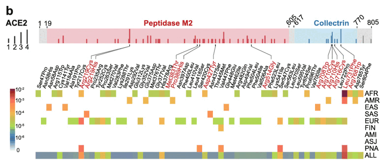
Specifically, 39% (24/61) and 54% (33/61) of deleterious variants in ACE2 occur in African/African-American (AFR) and Non-Finnish European (EUR) populations, respectively (Fig. 1b). Prevalence of deleterious variants among Latino/Admixed American (AMR), East Asian (EAS), Finnish (FIN), and South Asian (SAS) populations is 2-10%, while Amish (AMI) and Ashkenazi Jewish (ASJ) populations do not appear to carry such variants in ACE2 coding regions (Fig. 1b).

Figure 1b shows that the number of deleterious ACE2 alleleles which occurred at least once was 0 in Ashkenazis and Amishes, 1 in Finns, 2 in South Asians, and so on:

However there's a bias where populations with a larger sample size are more likely to have one or more occurrence of a deleterious allele than populations with a smaller sample size. In gnomAD v3 which was used in the paper, some populations have a much smaller population size than other populations, so for example the number of samples that have been typed for the K26R allele of ACE2 is 53,215 for the population labeled "European (non-Finnish)" but only 2,650 for Ashkenazis and 684 for Amishes. [https://gnomad.broadinstitute.org/variant/X-15600835-T-C?dataset=gnomad_r3] So the small population size explains why Ashkenazis and Amishes had zero occurrences of the deleterious alleles.

You can see the frequency of ACE2 alleles in gnomAD v3 from here: https://gnomad.broadinstitute.org/gene/ENSG00000130234?dataset=gnomad_r3. Then if you click "Export variants to CSV", you can run the following R code to count how many alleles each population had that were classified as deleterious in the paper that was linked by RFK:

> al=strsplit("Ser47Pro Asn58His Asn58Asp Arg115Trp Cys141Tyr Val184Ala Ala191Pro Tyr217Cys Arg219Cys Arg219His Pro235Arg Tyr252Cys Pro263Ser Met270Val Val283Phe Lys288Thr Ile291Lys Asp292Val Glu312Lys Gly352Val Glu375Asp Met376Thr Gly377Val His378Arg Met383Thr Pro389His Asn397Asp Phe400Leu Leu410Val Leu418Ser Ser420Cys Asp427Tyr Asn437Ser Thr445Met Val447Phe Gly448Glu Met462Ile Arg482Gln Asp494Val Phe504Leu Phe504Ile Val506Ala Arg514Gly Phe523Leu Lys541Ile Ser547Cys Ser563Leu Leu570Ser Leu595Val Tyr654Ser Pro696Thr Val700Ile Arg708Trp Arg710Cys Arg710His Arg716Cys Leu722Pro Leu731Phe Arg768Trp Asp785Tyr Ser804Phe"," ")[[1]]
> t=read.csv("gnomAD_v3.1.2_ENSG00000130234_2023_07_18_20_18_13.csv",check.names=F)
> rows=na.omit(match(paste0("p.",al),t$`HGVS Consequence`))
> total=colSums(t[rows,grepl("Allele Number ",colnames(t))])
> deleterious=colSums(t[rows,grepl("Allele Count ",colnames(t))])
> o=data.frame(row.names=sub("Allele Number ","",names(total)),deleterious,total,ratio=deleterious/total)
> o=o[order(o$ratio),];o$ratio=sprintf("%.7f",o$ratio);o
                         deleterious   total     ratio
Amish                              0   41769 0.0000000
Middle Eastern                     0   14554 0.0000000
Ashkenazi Jewish                   0  161388 0.0000000
European (Finnish)                 1  367360 0.0000027
South Asian                        3  162912 0.0000184
East Asian                         5  218231 0.0000229
Latino/Admixed American           19  640622 0.0000297
European (non-Finnish)           136 3241463 0.0000420
Other                              6   91784 0.0000654
African/African American         455 1873327 0.0002429

So basically the output above shows that the total number of deleterious alleles is so miniscule that it won't make much difference.

If you look at TMPRSS2 instead of ACE2, the total number of alleles that were classified as deleterious is about 2 orders of magnitude bigger, and the ratio of deleterious alleles is the lowest in Ashkenazis and the highest in Finns:

> al=strsplit("Gly6Arg Tyr20Cys Glu23Ala Tyr37Cys Pro54Leu Thr58Met Leu91Gln Leu91Pro Gly142Arg Gly142Trp Asp144Glu Glu145Lys Cys148Phe Arg150Leu Val160Met Val171Met Gly181Arg Gly189Ala Gly189Cys Tyr190Asp Cys231Ser Leu239Phe Arg240Cys Arg255Ser Val257Met Gly259Ser Ala262Val Trp267Arg Gly282Arg Ile286Phe Thr287Pro Val292Met Ala295Gly Cys297Ser Val298Met Tyr322Cys His334Leu Pro335Leu Ser339Phe Ala347Glu Ala347Thr Ala347Val Phe357Ser Val364Ala Val364Leu Gly370Ser Gly383Arg Trp384Leu Thr387Ala Gly391Glu Ile405Thr Met424Val Gly432Ala Gly432Glu Asp435Tyr Gln438Glu Pro444Leu Gly457Arg Ser460Arg Gly462Asp Gly462Ser Cys465Tyr Arg470Ile"," ")[[1]]
> t=read.csv("gnomAD_v3.1.2_ENSG00000184012_2023_07_18_23_46_03.csv",check.names=F)
> rows=na.omit(match(paste0("p.",al),t$`HGVS Consequence`))
> total=colSums(t[rows,grepl("Allele Number ",colnames(t))])
> deleterious=colSums(t[rows,grepl("Allele Count ",colnames(t))])
> o=data.frame(row.names=sub("Allele Number ","",names(total)),deleterious,total,ratio=deleterious/total)
> o=o[order(o$ratio),];o$ratio=sprintf("%.7f",o$ratio);o
                         deleterious   total     ratio
Ashkenazi Jewish                 493  214382 0.0022996
Latino/Admixed American         2436  943212 0.0025827
Middle Eastern                    56   19498 0.0028721
Other                            430  128910 0.0033357
European (non-Finnish)         15547 4200196 0.0037015
South Asian                     1157  297238 0.0038925
Amish                            234   56286 0.0041573
African/African American       12223 2557968 0.0047784
East Asian                      2007  320878 0.0062547
European (Finnish)              4172  653440 0.0063847

However almost all of the difference in the number of deleterious TMPRSS2 alleles is accounted by Val160Met, which has a minor allele frequency ranging from about 14% in Ashkenazis to about 39% in Finns:

So if the Val160Met allele does not actually have that much impact on suspectibility to COVID, then Ashkenazis may not have a significant advantage in terms of their profile of TMPRSS2 alleles either. And actually if Val160Met is excluded, then Ashkenazis have the second-highest ratio of deleterious TMPRSS2 alleles in gnomAD v3:

                         deleterious   total     ratio
Amish                              0   55378 0.0000000
Middle Eastern                     0   19182 0.0000000
European (Finnish)                 3  642848 0.0000047
East Asian                         3  315700 0.0000095
South Asian                        3  292408 0.0000103
European (non-Finnish)            61 4132214 0.0000148
Other                              4  126818 0.0000315
Latino/Admixed American           35  927936 0.0000377
Ashkenazi Jewish                  15  210912 0.0000711
African/African American         304 2516608 0.0001208

Paper about ACE2 by Ali et al.

Another paper which has been used as a source for the claim that Ashkenazis are less suspectible to COVID than other ethnic groups is a paper by Ali et al. from 2020 titled "ACE2 coding variants in different populations and their potential impact on SARS-CoV-2 binding affinity". [https://www.ncbi.nlm.nih.gov/pmc/articles/PMC7439997/] The paper only looked at a handful of ACE2 mutations, but the paper that RFK linked looked at a larger number of mutations of both ACE2 and TMPRSS2.

The part of the paper that conspiratards focused on was the figure shown below, which lists the 6 alleles that were analyzed in the paper so that they are ordered by their modeled level of electrostatic interaction with the spike protein of SARS-CoV-2. The K26R allele which is the most common in Ashkenazis has a red background because it's the only allele which was modeled as beneficial, but the other 5 alleles were modeled as detrimental so they have a green background:

In the figure above, East Asians are shown to have the highest frequency of the I468V allele, which was modeled as the least harmful of the 5 deleterious alleles, and which some people thought meant that East Asians would have the second-most advantageous mutation profile after Ashkenazis. But actually even though the I468V allele is modeled as only mildly deleterious in the paper, and even though only about 1.1% of East Asians have the allele at gnomAD v2, the other deleterious alleles analyzed in the paper are also so rare that if you calculate a weighted average of the frequency of each allele at gnomAD multiplied by the modeled interaction energy of each mutated form of ACE2, then East Asians end up having the lowest total interaction energy level, which might theoretically make them the most suspectible to COVID. But all 6 alleles listed in the paper are so rare that there's only a tiny range of variation in the weighted averages of the energy levels, so that they range from about -40.222 kcal/mol in East Asians to about -40.175 kcal/mol in Ashkenazis:
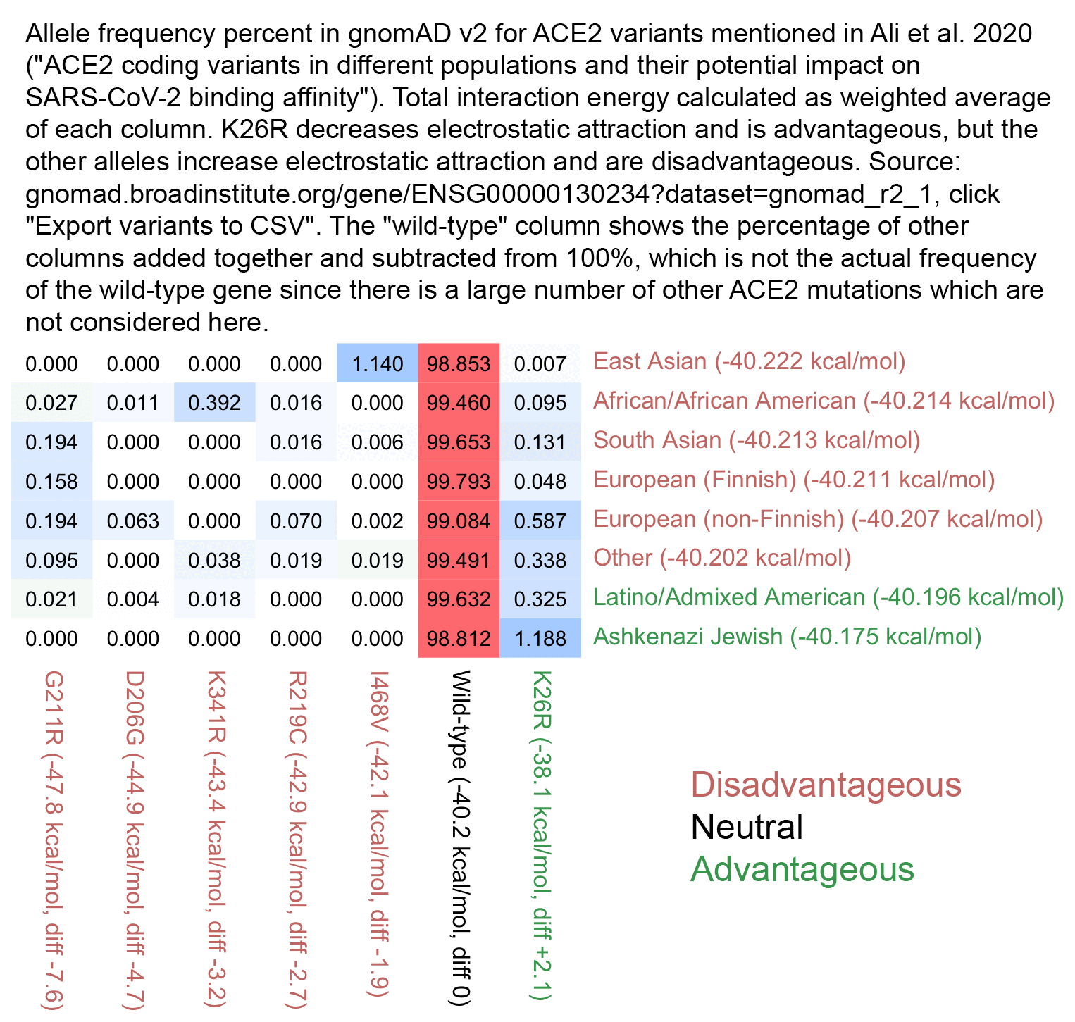
Here's R code to reproduce the plot above:

# install.packages("BiocManager")
# BiocManager::install("ComplexHeatmap")
# install.packages("circlize"
# install.packages("colorspace")
library(ComplexHeatmap)
library(circlize) # for colorRamp2
library(colorspace)

native=-40.2

energy=read.csv(header=F,text="G211R,-47.8
D206G,-44.9
K341R,-43.4
R219C,-42.9
I468V,-42.1
K26R,-38.1")

codon=read.csv(header=F,row.names=1,text="A,Ala
C,Cys
D,Asp
E,Glu
F,Phe
G,Gly
H,His
I,Ile
K,Lys
L,Leu
M,Met
N,Asn
P,Pro
Q,Gln
R,Arg
S,Ser
T,Thr
V,Val
W,Trp
X,Ter
Y,Tyr")

# freq=read.csv("gnomAD_v2.1.1_ENSG00000130234_2023_07_18_15_15_32.csv",check.names=F) # go to https://gnomad.broadinstitute.org/gene/ENSG00000130234?dataset=gnomad_r2_1 and click "Export variants to CSV"
freq=read.csv("https://pastebin.com/raw/sqKQ7Lk7",check.names=F)

name=paste0("p.",codon[substr(energy[,1],1,1),],sub(".(.*).","\\1",energy[,1]),codon[sub(".*(.)","\\1",energy[,1]),])
rows=match(name,freq$`HGVS Consequence`)

freq1=freq[rows,grepl("Allele Number ",colnames(freq))]
freq2=freq[rows,grepl("Allele Count ",colnames(freq))]

diff=round(energy[,2]-native,1)
diff=ifelse(diff>0,paste0("+",diff),diff)

m=freq2/freq1
sums=(1-colSums(m))*native+colSums(m*energy[,2])
rownames(m)=paste0(energy[,1]," (",energy[,2]," kcal/mol, diff ",diff,")")
colnames(m)=paste0(sub("Allele Number ","",colnames(freq1))," (",sprintf("%.3f",sums)," kcal/mol)")
m=m[,order(sums)]
m=rbind(m,1-colSums(m))

rownames(m)[nrow(m)]="Wild type (-40.2 kcal/mol, diff 0)"
m=m[c(1:5,7,6),]

m=t(m)*100
disp=apply(m,2,sprintf,fmt="%.3f")
m=sqrt(m)
m[is.na(m)]=0

colcol=hcl(c(0,0,0,0,0,0,120)+15,c(60,60,60,60,60,0,60),c(60,60,60,60,60,0,60))
rowcol=hcl(c(0,0,0,0,0,0,120,120)+15,60,60)

maxcolor=max(m)

png("1.png",w=ncol(m)*60+2000,h=nrow(m)*60+2000,res=144)
ht_opt$COLUMN_ANNO_PADDING=unit(0,"mm")
ht_opt$ROW_ANNO_PADDING=unit(0,"mm")

Heatmap(
  m,
  show_heatmap_legend=F,
  show_column_names=F,
  show_row_names=F,
  width=unit(ncol(m)*58,"pt"),
  height=unit(nrow(m)*28,"pt"),
  cluster_columns=F,
  cluster_rows=F,
  na_col="white",
  rect_gp=gpar(col="gray80",lwd=0),
  bottom_annotation=columnAnnotation(text=anno_text(gt_render(colnames(m),padding=unit(c(3,3,3,3),"mm")),just="left",rot=270,gp=gpar(fontsize=17,col=colcol))),
  right_annotation=rowAnnotation(text=anno_text(gt_render(rownames(m),padding=unit(c(3,3,3,3),"mm")),just="left",location=unit(0,"npc"),gp=gpar(fontsize=17,col=rowcol,border="gray70",lwd=0))),
  col=colorRamp2(seq(0,maxcolor,,7),colorspace::hex(colorspace::HSV(c(210,210,130,60,40,20,0),c(0,.5,.5,.5,.5,.5,.5),1))),
  cell_fun=\(j,i,x,y,w,h,fill)grid.text(disp[i,j],x,y,gp=gpar(fontsize=15,col="black"))
)

dev.off()
system("mogrify -gravity center -trim -border 16 -bordercolor white 1.png")

From the figure by Ali et al. I showed above, it's not clear that even though the K26R allele is the most common in Ashkenazis out of the handful of populations at gnomAD, the frequency of the allele in Ashkenazis is still only about 1.2% in gnomAD v2 and about 1.3% in gnomAD v3, so it won't give Ashkenazis any kind of a major advantage. [https://gnomad.broadinstitute.org/variant/X-15618958-T-C?dataset=gnomad_r2_1, https://gnomad.broadinstitute.org/variant/X-15600835-T-C?dataset=gnomad_r3] This table shows the frequency of the SNP which produces the K26R allele at gnomAD v2.1.1:

There's only a small number of populations at gnomAD, and other populations that are missing from gnomAD might have a higher frequency of the K26R allele than Ashkenazis. In Supplementary Table 1 from Ali et al. which is shown below, the frequencies of the ACE2 alleles are also reported among samples from 1000 Genomes, but the populations at 1000 Genomes are aggregated into continental groups so you can't see the results of individual ethnic groups apart from Han Chinese. It's probably because 1000 Genomes only has around a hundred or fewer samples per ethnic group, so the sample sizes are too small to accurately estimate the frequency of alleles that only appear in less than 1% or 0.1% of the population:

The K26R allele might be detrimental and not advantageous

Even though the K26R mutation was modeled as beneficial in the paper by Ali et al., it was modeled as detrimental in two other papers (from the point of views of humans who wish to avoid getting infected with the virus and not from the point of view of the virus).

In the other paper titled "New insights into genetic susceptibility of COVID-19: an ACE2 and TMPRSS2 polymorphism analysis", the authors wrote: [https://www.ncbi.nlm.nih.gov/pmc/articles/PMC7654750/]

Three SNVs, E329G (rs143936283), M82I (rs267606406) and K26R (rs4646116), had a significant reduction in binding free energy, which indicated higher binding affinity than wild-type ACE2 and greater susceptibility to SARS-CoV-2 infection for people with them.

And in the other paper titled "Molecular simulation of SARS-CoV-2 spike protein binding to pangolin ACE2 or human ACE2 natural variants reveals altered susceptibility to infection", the authors wrote: [https://www.ncbi.nlm.nih.gov/pmc/articles/PMC7843038/]

The K26, which is just proximal to the first region of the ACE2 receptor involved in S-protein binding, has been shown previously to bind the sterically hindering first mannose in the glycan that is linked to N90 and thus stabilizes the glycan moiety hindering the binding of S-protein RBD to ACE2 [41] (Figure 2A). The missense variant R26 creates a new hydrogen bond with D30, which is then poised to build a salt-bridge with the S-protein RBD K417 that increases the affinity of SARS-CoV-2 to the ACE2 receptor [21] (Figure 2B). Indeed, the ACE2 K26R activating variant was extremely rare in East Asian (MAF = 0.007%), Africans (MAF = 0.095%), but the second most common variant in Europeans with MAF of 0.587% (shown in green fonts in Table 1). The MAF of this variant in the Kuwaiti population was nearly half that of Europeans (MAF = 0.29%), and it was absent from the Qatari and Iranian exome data (Table 1). Our structural modeling supports the notion that K26R is an ACE2 receptor activating variant (Figure 2A, B). Consistent with these findings, using a synthetic human ACE2 mutant library, a recent study reported that the R26 variant increased S-protein binding and susceptibility to the virus significantly [42].

Frequency of the TMPRSS2 Val160Met allele in the Reich dataset

The Reich dataset is a collection of over 10,000 ancient and modern human genetic samples. [https://reich.hms.harvard.edu/allen-ancient-dna-resource-aadr-downloadable-genotypes-present-day-and-ancient-dna-data] Viruses have such short genomes that it's easy to do genetic analysis of viruses using whole genome sequences, but humans have much longer genomes and there is little variation between humans for the vast majority of nucleotide positions, so in human population genetics it's common to only analyze subsets of SNPs which have a considerable level of variation across humans. One subset of SNPs that is used by the Reich dataset is called the 1240K panel, and it includes about 1.2 million SNPs. So the Reich dataset is essentially a table which has over 10,000 rows for different human genetic samples, and it has about 1.2 million columns for each SNP which indicate whether each sample has 0, 1, or 2 copies of the SNP (even though there is also another version of the dataset which only has about 600,000 SNPs but which includes a larger number of present-day samples in addition to ancient samples).

In the paper about ACE2 and TMPRSS alleles that RFK linked on his Substack, the only allele with a high minor allele frequency was the Val160Met allele of the TMPRSS2 gene. The allele is produced by the rs12329760 SNP, which is included in the 1240K SNP panel. I calculated the frequency of the SNP in populations of the Reich dataset that have at least 20 samples that are not missing data for the SNP. The modern populations with the lowest frequency for the SNP were Peruvians, Bedouins from Israel, and Mozabite Berbers. However Ashkenazis or other Jewish populations are not included, because I used the 1240K version of the Reich dataset which has a small number of present-day samples, but the allele still appears to be less common in Mediterranean populations than in Northern Europeans, East Asians, or sub-Saharan Africans:

$ brew install plink2
[...]
$ curl https://github.com/chrchang/eigensoft/raw/master/mac/convertf>/usr/local/bin/convertf;chmod +x /usr/local/bin/convertf
$ wget https://reichdata.hms.harvard.edu/pub/datasets/amh_repo/curated_releases/V54/V54.1.p1/SHARE/public.dir/v54.1.p1_1240K_public.{anno,ind,snp,geno}
$ x=v54.1.p1_1240K_public;convertf -p <(printf %s\\n genotypename:\ $x.geno snpname:\ $x.snp indivname:\ $x.ind outputformat:\ PACKEDPED genotypeoutname:\ $x.bed snpoutname:\ $x.bim indivoutname:\ $x.fam)
[...]
$ plink2 --bfile v54.1.p1_1240K_public --extract <(echo rs12329760) --recode A
[...]
$ printf %s\\n 'ACB.SG;Afro-Caribbean, Barbados' 'ASW.SG;African-American' 'BEB.SG;Bangladesh' 'CDX.SG;Chinese Dai' 'CEU.SG;Utah white' 'CHB.SG;Han, Beijing' 'CHS.SG;Southern Han' 'CLM.SG;Medellin, Colombia' 'ESN.SG;Esan, Nigeria' 'FIN.SG;Finnish' 'GBR.SG;British' 'GIH.SG;Gujaratis, Houston' 'GWD.SG;Gambia, Western Divisions' 'IBS_CanaryIslands.SG;Canary Islands' 'IBS.SG;Spanish' 'ITU.SG;Telugu, United Kingdom' 'JPT.SG;Japanese' 'KHV.SG;Vietnamese' 'LWK.SG;Kenya, Webuye' 'MSL.SG;Mende, Sierra Leone' 'MXL.SG;Mexican-American, Los Angeles' 'PEL.SG;Peru, Lima' 'PJL.SG;Pakistan, Punjab Lahore' 'PUR.SG;Puerto Rico' 'STU.SG;Tamils, United Kingdom' 'TSI.SG;Italy, Tuscany' 'YRI.SG;Yoruba'>1kgpop
$ awk '$7!="NA"{n[$1]++;c[$1]+=$7}END{for(i in n)if(n[i]>=20)print i,100*c[i]/n[i]/2,c[i],2*n[i]}' plink.raw|sort -rnk2|awk '{$2=sprintf("%.1f",$2)}1'|tr \  \;|awk 'NR==FNR{a[$1]=$2;next}$1 in a{$1="1KG: "a[$1]}1' {,O}FS=\; 1kgpop -|(echo 'population;pct;deleterious;total';cat)|column -ts\;
population                          pct   deleterious  total
USA_MarianaIslands_Latte            56.4  44           78
1KG: Japanese                       45.4  88           194
Guam_Latte                          43.9  50           114
1KG: Finnish                        42.7  76           178
1KG: Han, Beijing                   39.8  78           196
1KG: Southern Han                   39.6  80           202
Han.SDG                             39.3  33           84
Estonia_EarlyViking.SG              37.5  24           64
1KG: Chinese Dai                    37.2  73           196
Serbia_IronGates_Mesolithic         36.4  16           44
1KG: Gambia, Western Divisions      35.7  80           224
Japanese.SDG                        35.2  19           54
1KG: Mende, Sierra Leone            33.3  56           168
1KG: Kenya, Webuye                  33.3  62           186
1KG: Vietnamese                     33.0  64           194
Brahui.SDG                          31.8  14           44
1KG: African-American               31.6  36           114
1KG: Afro-Caribbean, Barbados       30.4  56           184
Yakut.SDG                           30.0  12           40
1KG: Bangladesh                     29.8  50           168
1KG: Tamils, United Kingdom         29.3  58           198
England_Viking.SG                   28.6  12           42
1KG: Yoruba                         27.7  52           188
Spain_C                             27.3  12           44
Czech_CordedWare                    27.3  18           66
Russian.SDG                         27.1  13           48
England_MIA_LIA                     26.2  22           84
Czech_IA_LaTene                     26.1  12           46
1KG: Mexican-American, Los Angeles  25.8  32           124
England_MIA                         25.7  36           140
Czech_BellBeaker                    25.7  18           70
1KG: Pakistan, Punjab Lahore        25.0  48           192
England_EastYorkshire_MIA_LIA       25.0  12           48
1KG: Esan, Nigeria                  24.5  48           196
Scotland_N                          24.1  14           58
Croatia_C_Lasinja                   24.0  12           50
Yoruba.SDG                          23.8  10           42
1KG: Italy, Tuscany                 23.6  50           212
Sweden_Viking.SG                    23.5  40           170
1KG: Utah white                     22.2  44           198
1KG: British                        20.9  38           182
1KG: Medellin, Colombia             20.7  38           184
1KG: Spanish                        20.6  42           204
Denmark_Viking.SG                   20.5  18           88
Italy_Imperial.SG                   20.0  8            40
1KG: Telugu, United Kingdom         19.6  40           204
Czech_EBA_Unetice                   19.3  32           166
Germany_BellBeaker                  19.0  8            42
Palestinian.SDG                     18.6  13           70
France_MN                           18.2  8            44
Norway_Viking.SG                    17.6  12           68
1KG: Gujaratis, Houston             17.6  36           204
Balochi.SDG                         17.5  7            40
1KG: Puerto Rico                    16.3  32           196
Switzerland_LN                      15.0  6            40
England_EIA                         15.0  6            40
Basque.SDG                          14.3  6            42
Sardinian.SDG                       14.0  7            50
Burusho.SDG                         13.6  6            44
Kalash.SDG                          11.9  5            42
Iceland_Viking.SG                   10.0  4            40
French.SDG                          10.0  5            50
Druze.SDG                           9.0   7            78
Makrani.SDG                         7.5   3            40
Cuba_CanimarAbajo_Archaic           5.3   4            76
England_C_EBA                       4.8   2            42
Mozabite.SDG                        4.5   2            44
Pakistan_Loebanr_IA                 4.3   2            46
BedouinA.SDG                        4.0   2            50
1KG: Peru, Lima                     2.9   4            138
Germany_EN_LBK                      0.0   0            42
Dominican_LaCaleta_Ceramic          0.0   0            72

When I searched for studies about the Val160Met allele, I found a paper titled "Initial study on TMPRSS2 p.Val160Met genetic variant in COVID-19 patients", where the authors found that people with the Val160Met mutation had a higher viral load and a higher mortality rate than people without the mutation, but the sample size of the study was only 95 so the findings may have been due to chance: [https://www.ncbi.nlm.nih.gov/pmc/articles/PMC8127183/]

We genotyped 95 patients with COVID-19 hospitalised in Dr Soetomo General Hospital and Indrapura Field Hospital (Surabaya, Indonesia) for the TMPRSS2 p.Val160Met polymorphism. Polymorphism was detected using a TaqMan assay. We then analysed the association between the presence of the genetic variant and disease severity and viral load. We did not observe any correlation between the presence of TMPRSS2 genetic variant and the severity of the disease. However, we identified a significant association between the p.Val160Met polymorphism and the SARS-CoV-2 viral load, as estimated by the Ct value of the diagnostic nucleic acid amplification test. Furthermore, we observed a trend of association between the presence of the C allele and the mortality rate in patients with severe COVID-19.

Calculating a polygenic score for SNPs identified in a COVID GWAS

When I searched for genome-wide association studies about COVID, I found a paper titled "Genetic variants are identified to increase risk of COVID-19 related mortality from UK Biobank data": [https://www.ncbi.nlm.nih.gov/pmc/articles/PMC7856608/]

Methods

In this project, we consider the mortality as the trait of interest and perform a genome-wide association study (GWAS) of data for 1778 infected cases (445 deaths, 25.03%) distributed by the UK Biobank. Traditional GWAS fails to identify any genome-wide significant genetic variants from this dataset. To enhance the power of GWAS and account for possible multi-loci interactions, we adopt the concept of super variant for the detection of genetic factors. A discovery-validation procedure is used for verifying the potential associations.

Results

We find 8 super variants that are consistently identified across multiple replications as susceptibility loci for COVID-19 mortality. The identified risk factors on chromosomes 2, 6, 7, 8, 10, 16, and 17 contain genetic variants and genes related to cilia dysfunctions (DNAH7 and CLUAP1), cardiovascular diseases (DES and SPEG), thromboembolic disease (STXBP5), mitochondrial dysfunctions (TOMM7), and innate immune system (WSB1). It is noteworthy that DNAH7 has been reported recently as the most downregulated gene after infecting human bronchial epithelial cells with SARS-CoV-2.

The super-variants that were discovered in the study had a huge effect on mortality, so for example in people with the super-variant chr17_26, the risk of dying within a month from a positive COVID test was almost 40%, which was more than double the average risk within the patient population that was included in the study. So the effect of the super-variants is probably a lot bigger than the effect of the ACE2 or TMPRSS2 mutations that were analyzed in the other papers:

There were a total of 23 SNPs associated with the 8 "super-variants", so I scraped gnomAD's website for the allele frequency table of all 23 SNPs, and I calculated a sum of the frequency of each SNP multiplied by its odds ratio listed in the paper (which I know is not the correct way to calculate a polygenic score, but you'll have to deal with my redneck methodology). But anyway, East Asians had the highest score, where a higher score means a more deleterious profile of alleles, and Ashkenazis had the second-lowest score after non-Finnish-non-Ashkenazi Europeans:

$ Rscript -e 't=read.csv("supervariants.csv");t=t[t$allele_number!=0,];o=round(sort(tapply(t$odds_ratio*t$allele_count/t$allele_number,t$population,sum)),2);writeLines(paste(o,names(o)))'
5.51 European (non-Finnish)
5.59 Ashkenazi Jewish
6.08 Other
6.28 African/African American
6.67 European (Finnish)
7.28 Latino/Admixed American
9.04 East Asian
$ cat supervariants.csv
snp,odds_ratio,population,allele_count,allele_number
rs73060484,1.945,Latino/Admixed American,215,846
rs73060484,1.945,East Asian,338,1558
rs73060484,1.945,European (Finnish),564,3472
rs73060484,1.945,Other,125,1088
rs73060484,1.945,African/African American,882,8702
rs73060484,1.945,Ashkenazi Jewish,23,290
rs73060484,1.945,European (non-Finnish),1066,15422
rs73060484,1.945,South Asian,0,0
rs77578623,1.939,Latino/Admixed American,203,796
rs77578623,1.939,East Asian,334,1532
rs77578623,1.939,European (Finnish),487,3016
rs77578623,1.939,Other,117,1014
rs77578623,1.939,African/African American,844,8402
rs77578623,1.939,Ashkenazi Jewish,23,288
rs77578623,1.939,European (non-Finnish),1026,14960
rs77578623,1.939,South Asian,0,0
rs74417002,1.832,African/African American,543,8700
rs74417002,1.832,European (non-Finnish),398,15418
rs74417002,1.832,Other,20,1086
rs74417002,1.832,Ashkenazi Jewish,5,290
rs74417002,1.832,Latino/Admixed American,13,848
rs74417002,1.832,European (Finnish),40,3472
rs74417002,1.832,East Asian,0,1560
rs74417002,1.832,South Asian,0,0
rs73070529,2.249,Latino/Admixed American,214,844
rs73070529,2.249,East Asian,296,1546
rs73070529,2.249,African/African American,1648,8628
rs73070529,2.249,European (Finnish),281,3462
rs73070529,2.249,Other,84,1074
rs73070529,2.249,Ashkenazi Jewish,19,290
rs73070529,2.249,European (non-Finnish),666,15320
rs73070529,2.249,South Asian,0,0
rs113892140,2.031,Latino/Admixed American,209,846
rs113892140,2.031,African/African American,1928,8600
rs113892140,2.031,East Asian,298,1548
rs113892140,2.031,European (Finnish),280,3438
rs113892140,2.031,Other,86,1074
rs113892140,2.031,Ashkenazi Jewish,12,288
rs113892140,2.031,European (non-Finnish),612,15238
rs113892140,2.031,South Asian,0,0
rs200008298,1.8,Ashkenazi Jewish,9,290
rs200008298,1.8,European (Finnish),100,3472
rs200008298,1.8,European (non-Finnish),420,15414
rs200008298,1.8,Other,25,1084
rs200008298,1.8,African/African American,135,8712
rs200008298,1.8,Latino/Admixed American,8,846
rs200008298,1.8,East Asian,0,1560
rs200008298,1.8,South Asian,0,0
rs183712207,4.783,European (Finnish),232,3466
rs183712207,4.783,Other,26,1084
rs183712207,4.783,European (non-Finnish),213,15376
rs183712207,4.783,Latino/Admixed American,10,848
rs183712207,4.783,African/African American,38,8690
rs183712207,4.783,East Asian,1,1556
rs183712207,4.783,Ashkenazi Jewish,0,290
rs183712207,4.783,South Asian,0,0
rs191631470,3.335,European (Finnish),234,3474
rs191631470,3.335,Other,26,1088
rs191631470,3.335,European (non-Finnish),212,15428
rs191631470,3.335,Latino/Admixed American,10,846
rs191631470,3.335,Ashkenazi Jewish,2,290
rs191631470,3.335,African/African American,24,8716
rs191631470,3.335,East Asian,0,1560
rs191631470,3.335,South Asian,0,0
rs2176724,1.484,African/African American,3047,8654
rs2176724,1.484,Ashkenazi Jewish,33,290
rs2176724,1.484,Other,122,1086
rs2176724,1.484,European (non-Finnish),1708,15372
rs2176724,1.484,Latino/Admixed American,71,838
rs2176724,1.484,European (Finnish),243,3458
rs2176724,1.484,East Asian,1,1556
rs2176724,1.484,South Asian,0,0
rs71040457,1.331,East Asian,1249,1532
rs71040457,1.331,European (Finnish),2480,3428
rs71040457,1.331,European (non-Finnish),9731,15106
rs71040457,1.331,Latino/Admixed American,538,840
rs71040457,1.331,Other,681,1064
rs71040457,1.331,Ashkenazi Jewish,154,286
rs71040457,1.331,African/African American,1332,8596
rs71040457,1.331,South Asian,0,0
rs117928001,2.749,European (non-Finnish),956,15428
rs117928001,2.749,Other,41,1088
rs117928001,2.749,European (Finnish),129,3472
rs117928001,2.749,Latino/Admixed American,26,848
rs117928001,2.749,Ashkenazi Jewish,7,290
rs117928001,2.749,African/African American,88,8700
rs117928001,2.749,East Asian,1,1560
rs117928001,2.749,South Asian,0,0
rs116898161,2.541,European (non-Finnish),905,15416
rs116898161,2.541,European (Finnish),128,3468
rs116898161,2.541,Other,39,1084
rs116898161,2.541,Latino/Admixed American,25,846
rs116898161,2.541,Ashkenazi Jewish,7,290
rs116898161,2.541,African/African American,73,8710
rs116898161,2.541,East Asian,1,1560
rs116898161,2.541,South Asian,0,0
rs13227460,1.3,European (Finnish),923,3412
rs13227460,1.3,European (non-Finnish),4084,15278
rs13227460,1.3,Latino/Admixed American,183,842
rs13227460,1.3,Other,229,1072
rs13227460,1.3,Ashkenazi Jewish,48,290
rs13227460,1.3,East Asian,221,1558
rs13227460,1.3,African/African American,699,8684
rs13227460,1.3,South Asian,0,0
rs55986907,1.601,Ashkenazi Jewish,107,286
rs55986907,1.601,Latino/Admixed American,312,846
rs55986907,1.601,European (Finnish),1076,3468
rs55986907,1.601,European (non-Finnish),4522,15376
rs55986907,1.601,Other,314,1088
rs55986907,1.601,East Asian,263,1560
rs55986907,1.601,African/African American,1247,8686
rs55986907,1.601,South Asian,0,0
rs7817272,1.736,East Asian,934,1552
rs7817272,1.736,African/African American,3130,8690
rs7817272,1.736,Latino/Admixed American,219,846
rs7817272,1.736,Other,253,1086
rs7817272,1.736,European (Finnish),798,3476
rs7817272,1.736,Ashkenazi Jewish,55,290
rs7817272,1.736,European (non-Finnish),2833,15404
rs7817272,1.736,South Asian,0,0
rs4735444,1.784,East Asian,931,1554
rs4735444,1.784,African/African American,2991,8694
rs4735444,1.784,Latino/Admixed American,218,848
rs4735444,1.784,Other,253,1086
rs4735444,1.784,Ashkenazi Jewish,67,290
rs4735444,1.784,European (Finnish),782,3472
rs4735444,1.784,European (non-Finnish),2928,15416
rs4735444,1.784,South Asian,0,0
rs2874140,1.694,East Asian,947,1552
rs2874140,1.694,African/African American,3404,8674
rs2874140,1.694,Latino/Admixed American,216,846
rs2874140,1.694,Other,258,1086
rs2874140,1.694,European (Finnish),794,3458
rs2874140,1.694,Ashkenazi Jewish,57,286
rs2874140,1.694,European (non-Finnish),2838,15376
rs2874140,1.694,South Asian,0,0
rs7007951,1.711,East Asian,927,1556
rs7007951,1.711,African/African American,2945,8700
rs7007951,1.711,Latino/Admixed American,214,848
rs7007951,1.711,Other,245,1086
rs7007951,1.711,European (Finnish),771,3470
rs7007951,1.711,Ashkenazi Jewish,56,290
rs7007951,1.711,European (non-Finnish),2726,15412
rs7007951,1.711,South Asian,0,0
rs920576,1.615,East Asian,947,1550
rs920576,1.615,African/African American,2706,8676
rs920576,1.615,Latino/Admixed American,219,844
rs920576,1.615,Ashkenazi Jewish,70,290
rs920576,1.615,Other,259,1076
rs920576,1.615,European (Finnish),799,3460
rs920576,1.615,European (non-Finnish),2966,15398
rs920576,1.615,South Asian,0,0
rs9804218,1.373,Ashkenazi Jewish,192,248
rs9804218,1.373,European (non-Finnish),7912,12902
rs9804218,1.373,Other,553,942
rs9804218,1.373,European (Finnish),1752,3062
rs9804218,1.373,Latino/Admixed American,306,666
rs9804218,1.373,African/African American,3135,6942
rs9804218,1.373,East Asian,183,1448
rs9804218,1.373,South Asian,0,0
rs2301762,2.541,East Asian,281,1558
rs2301762,2.541,Latino/Admixed American,60,848
rs2301762,2.541,European (Finnish),226,3474
rs2301762,2.541,Other,66,1088
rs2301762,2.541,European (non-Finnish),886,15422
rs2301762,2.541,Ashkenazi Jewish,8,290
rs2301762,2.541,African/African American,105,8716
rs2301762,2.541,South Asian,0,0
rs60811869,2.966,European (non-Finnish),376,15432
rs60811869,2.966,African/African American,212,8714
rs60811869,2.966,Ashkenazi Jewish,7,290
rs60811869,2.966,Other,22,1088
rs60811869,2.966,Latino/Admixed American,17,848
rs60811869,2.966,European (Finnish),56,3476
rs60811869,2.966,East Asian,24,1558
rs60811869,2.966,South Asian,0,0
rs117217714,6.255,Ashkenazi Jewish,5,290
rs117217714,6.255,Other,10,1084
rs117217714,6.255,European (non-Finnish),134,15420
rs117217714,6.255,European (Finnish),12,3472
rs117217714,6.255,African/African American,15,8706
rs117217714,6.255,Latino/Admixed American,1,848
rs117217714,6.255,East Asian,0,1556
rs117217714,6.255,South Asian,0,0

However in order to accurately the estimate the suspectibility of different ethnic groups to COVID, you'd need to do a GWAS with a bigger sample size and you'd need to look at more than just 23 SNPs.